卷积神经网络训练过程中的training step的含义_TensorFlow2.0代码实战专栏(五):神经网络示例...

作者 | Aymeric Damien
编辑 | 奇予纪
出品 | 磐创AI团队
原项目 | https://github.com/aymericdamien/TensorFlow-Examples/
![]() AI学习路线之TensorFlow篇
AI学习路线之TensorFlow篇
神经网络示例
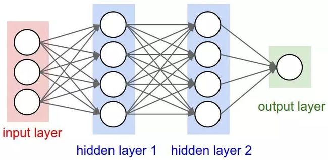
使用TensorFlow v2构建一个两层隐藏层完全连接的神经网络(多层感知器)。 这个例子使用低级方法来更好地理解构建神经网络和训练过程背后的所有机制。神经网络概述:
MNIST数据集概述:
此示例使用手写数字的MNIST数据集。 该数据集包含60,000个用于训练的示例和10,000个用于测试的示例。 这些数字已经过尺寸标准化并位于图像中心,图像是固定大小(28x28像素),值为0到255。 在此示例中,每个图像将转换为float32并归一化为[0,1],并展平为784个特征的一维数组(28 * 28)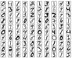
更多信息请查看链接: http://yann.lecun.com/exdb/mnist/
from __future__ import absolute_import, division, print_function

import tensorflow as tf
from tensorflow.keras import Model, layers
import numpy as np
# MNIST 数据集参数
num_classes = 10 # 所有类别(数字 0-9)
num_features = 784 # 数据特征数目 (图像形状: 28*28)

# 训练参数
learning_rate = 0.001
training_steps = 2000
batch_size = 256
display_step = 100

# 网络参数
n_hidden_1 = 128 # 第一层隐含层神经元的数目
n_hidden_2 = 256 # 第二层隐含层神经元的数目
# 准备MNIST数据
from tensorflow.keras.datasets import mnist
(x_train, y_train), (x_test, y_test) = mnist.load_data()
# 转化为float32
x_train, x_test = np.array(x_train, np.float32), np.array(x_test, np.float32)
# 将每张图像展平为具有784个特征的一维向量(28 * 28)
x_train, x_test = x_train.reshape([-1, num_features]), x_test.reshape([-1, num_features])
# 将图像值从[0,255]归一化到[0,1]
x_train, x_test = x_train / 255., x_test / 255.
# 使用tf.data API对数据进行随机排序和批处理
train_data = tf.data.Dataset.from_tensor_slices((x_train, y_train))
train_data = train_data.repeat().shuffle(5000).batch(batch_size).prefetch(1)
# 创建 TF 模型
class NeuralNet(Model):
    # 设置层
    def __init__(self):
        super(NeuralNet, self).__init__()
        # 第一层全连接隐含层
        self.fc1 = layers.Dense(n_hidden_1, activation=tf.nn.relu)
        # 第二层全连接隐含层
        self.fc2 = layers.Dense(n_hidden_2, activation=tf.nn.relu)
        # 全连接输出层
        self.out = layers.Dense(num_classes, activation=tf.nn.softmax)

    # 设置前向传播
    def call(self, x, is_training=False):
        x = self.fc1(x)
        x = self.out(x)
        if not is_training:
            # tf交叉熵期望输出没有softmax,所以只有
            #不训练时使用softmax。
            x = tf.nn.softmax(x)
        return x

# 构建神经网络模型
neural_net = NeuralNet()
# 交叉熵损失
# 注意这将会对输使用'softmax'
def cross_entropy_loss(x, y):

    # 将标签转化为int64以使用交叉熵函数
    y = tf.cast(y, tf.int64)
    #将softmax应用于输出并计算交叉熵。
    loss = tf.nn.sparse_softmax_cross_entropy_with_logits(labels=y, logits=x)
    # 批的平均损失。
    return tf.reduce_mean(loss)

# 准确率评估
def accuracy(y_pred, y_true):
    # 预测类是预测向量中最高分的索引(即argmax)
    correct_prediction = tf.equal(tf.argmax(y_pred, 1), tf.cast(y_true, tf.int64))
    return tf.reduce_mean(tf.cast(correct_prediction, tf.float32), axis=-1)

# 随机梯度下降优化器
optimizer = tf.optimizers.SGD(learning_rate)
# 优化过程
def run_optimization(x, y):
   # 将计算封装在GradientTape中以实现自动微分
    with tf.GradientTape() as g:
        # 前向传播
        pred = neural_net(x, is_training=True)
        # 计算损失
        loss = cross_entropy_loss(pred, y)

    # 要更新的变量,即可训练的变量
    trainable_variables = neural_net.trainable_variables

    # 计算梯度
    gradients = g.gradient(loss, trainable_variables)

    # 按gradients更新 W 和 b
    optimizer.apply_gradients(zip(gradients, trainable_variables))
# 针对给定步骤数进行训练
for step, (batch_x, batch_y) in enumerate(train_data.take(training_steps), 1):
    # 运行优化以更新W和b值
    run_optimization(batch_x, batch_y)

    if step % display_step == 0:
        pred = neural_net(batch_x, is_training=True)
        loss = cross_entrop

        ···y_loss(pred, batch_y)
        acc = accuracy(pred, batch_y)
        print("step: %i, loss: %f, accuracy: %f" % (step, loss, acc))
step: 100, loss: 2.031049, accuracy: 0.535156
step: 200, loss: 1.821917, accuracy: 0.722656
step: 300, loss: 1.764789, accuracy: 0.753906
step: 400, loss: 1.677593, accuracy: 0.859375
step: 500, loss: 1.643402, accuracy: 0.867188
step: 600, loss: 1.645116, accuracy: 0.859375
step: 700, loss: 1.618012, accuracy: 0.878906
step: 800, loss: 1.618097, accuracy: 0.878906
step: 900, loss: 1.616565, accuracy: 0.875000
step: 1000, loss: 1.599962, accuracy: 0.894531
step: 1100, loss: 1.593849, accuracy: 0.910156
step: 1200, loss: 1.594491, accuracy: 0.886719
step: 1300, loss: 1.622147, accuracy: 0.859375
step: 1400, loss: 1.547483, accuracy: 0.937500
step: 1500, loss: 1.581775, accuracy: 0.898438
step: 1600, loss: 1.555893, accuracy: 0.929688
step: 1700, loss: 1.578076, accuracy: 0.898438
step: 1800, loss: 1.584776, accuracy: 0.882812
step: 1900, loss: 1.563029, accuracy: 0.921875
step: 2000, loss: 1.569637, accuracy: 0.902344
# 在验证集上测试模型
pred = neural_net(x_test, is_training=False)
print("Test Accuracy: %f" % accuracy(pred, y_test)
# 可视化预测
import matplotlib.pyplot as plt
# 从验证集中预测5张图像
n_images = 5
test_images = x_test[:n_images]
predictions = neural_net(test_images)

# 显示图片和模型预测结果
for i in range(n_images):
    plt.imshow(np.reshape(test_images[i], [28, 28]), cmap='gray')
    plt.show()
    print("Model prediction: %i" % np.argmax(predictions.numpy()[i]))
output:
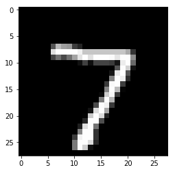 Model prediction: 7
  Model prediction:2
  Model prediction: 1
  Model prediction: 0
  Model prediction: 4
![]() 还想看更多TensorFlow2.0专栏文章?可在公众号底部菜单栏子菜单“独家原创”中找到TensorFlow2.0系列文章(如下图),同步更新中,关注公众号了解更多吧~
还想看更多TensorFlow2.0专栏文章?可在公众号底部菜单栏子菜单“独家原创”中找到TensorFlow2.0系列文章(如下图),同步更新中,关注公众号了解更多吧~

或点击下方“阅读原文”,进入TensorFlow2.0专栏,即可查看往期文章。
嗨,你还在看吗?