tensorflow 中的学习率衰减

在对一个模型进行训练时，通常建议随着训练的进行降低学习率，前期快速优化后期稳步收敛。设当前训练步数为 $global\_step$，初始学习率为 $learning\_rate$ 则学习率为：

$$current\_lr=decay\_fun(learning\_rate,global\_step,\theta )$$

衰减策略由函数 $decay\_fun$ 决定，其中 $\theta$ 为其他一些相关参数。

1. exponential_decay(指数衰减)

tf.train.exponential_decay(
    learning_rate,   # 初始学习率
    global_step,
    decay_steps,     # 指数函数的指数增长快慢
    decay_rate,      # 衰减率系数（指数函数的底数）
    staircase=False, # 是否是阶梯型衰减，默认是 False
    name=None
)

以 learning_rate 为初始值，学习率随 global_step 的增长呈指数下降，下降速度由 decay_rate（底数）和 decay_steps（决定指数增长速度）决定。公式：

$$current\_lr=learning\_rate\ast pow(decay\_rate,\frac{global\_step}{decay\_steps})$$

若 staircase=True，则 $\frac{global\_step}{decay\_steps}$ 取整数，学习率阶梯式下降（每隔 $decay\_steps$ 步下降一次），否则每一步都衰减。

使用示例：

import matplotlib.pyplot as plt
import tensorflow as tf

global_step = tf.Variable(0, name='global_step', trainable=False)
learning_rate_1 = tf.train.exponential_decay(  # 阶梯型衰减
	learning_rate=0.6, global_step=global_step, decay_steps=10,
	decay_rate=0.6,
	staircase=True
)
learning_rate_2 = tf.train.exponential_decay(  # 步步衰减
	learning_rate=0.6, global_step=global_step, decay_steps=10,
	decay_rate=0.6,
	staircase=False
)
add1 = tf.assign_add(global_step, 1)

steps, lrs_1, lrs_2 = [], [], []
with tf.Session() as sess:
	sess.run(tf.global_variables_initializer())
	for _ in range(60):
		current_step, current_lr_1, current_lr_2, _ = sess.run([global_step, learning_rate_1, learning_rate_2, add1])
		steps.append(current_step)
		lrs_1.append(current_lr_1)
		lrs_2.append(current_lr_2)

plt.plot(steps, lrs_1, 'r-', linewidth=2)
plt.plot(steps, lrs_2, 'g-', linewidth=2)
plt.title('exponential_decay')
plt.show()

exponential_decay 学习率衰减

红线表示阶梯式衰减（starecase=True），绿线表示步步衰减（starecase=False）。

2. piecewise_constant(分段常数衰减)

tf.train.piecewise_constant(
    x,           # global_step
    boundaries,  # List[int]，更新学习率的 step 边界
    values,      # lr_list，[base_lr, lr1, lr2, ...]
    name=None    # Defaults to 'PiecewiseConstant' 
)

人工指定学习率在哪些 step 衰减为何值。需提供额外参数：衰减步列表（boundaries），学习率列表（values）。

公式不好描述，用一个示意图表示 piecewise_constant

这个图中，线上是 current_lr，线下是 global_step，参数为

boundaries = [10, 20, 30, 40, 50]
values = [0.06, 0.05, 0.04, 0.03, 0.02, 0.01]

使用示例：

import matplotlib.pyplot as plt
import tensorflow as tf

global_step = tf.Variable(0, name='global_step', trainable=False)
learning_rate = tf.train.piecewise_constant(
	x=global_step,
	boundaries=[10, 20, 30, 40, 50],
	values=[0.06, 0.05, 0.04, 0.03, 0.02, 0.01]
)
add1 = tf.assign_add(global_step, 1)

steps, lrs = [], []
with tf.Session() as sess:
	sess.run(tf.global_variables_initializer())
	for _ in range(60):
		current_step, current_lr, _ = sess.run([global_step, learning_rate, add1])
		steps.append(current_step)
		lrs.append(current_lr)

plt.plot(steps, lrs, 'r-', linewidth=2)
plt.title('inverse_time_decay')
plt.show()

inverse_time_decay 学习率衰减

3. polynomial_decay(多项式衰减)

tf.train.polynomial_decay(
    learning_rate,  # 初始学习率
    global_step,
    decay_steps,  # 从 learning_rate 衰减到 end_learning_rate 的步数
    end_learning_rate=0.0001,  # 学习率更新到此停止
    power=1.0,   # 多项式指数，默认是线性的，取值为 1
    cycle=False, # 当超过 decay_steps 后是否循环执行
    name=None
)

学习率以 decay_steps 步，从 learning_rate 按多项式衰减到 end_learning_rate，当 cycle=True 时循环衰减。多项式为：

$$\begin{array}{rl}current\_lr& =(learning\_rate-end\_learning\_rate)\ast pow(1-\frac{global\_step}{decay\_steps},power)\\ & +end\_learning\_rate\end{array}$$

如果 cycle=False，则 $global\_step=min(global\_step,decay\_steps)$；
如果 cycle=True，则 $decay\_steps=decay\_steps\ast ceil(global\_step/decay\_steps)$，（从实验观察看，这个 $decay\_steps$ 不是递归的，$ceil$ 里的 $decay\_steps$ 是实参提供的初始的 $decay\_steps$）。所以[1]所说的周期变大理解是错误的，该博主理解成了递归。

使用示例：

import matplotlib.pyplot as plt
import tensorflow as tf

global_step = tf.Variable(0, name='global_step', trainable=False)
learning_rate_1 = tf.train.polynomial_decay(  # 非周期衰减
	learning_rate=0.102, global_step=global_step, decay_steps=10,
	end_learning_rate=0.011,  # 为了把线挪开一点分清，加了0.001
	power=1.0,
	cycle=False
)
learning_rate_2 = tf.train.polynomial_decay(  # 周期性衰减
	learning_rate=0.1, global_step=global_step, decay_steps=10,
	end_learning_rate=0.01,
	power=1.0,
	cycle=True
)
add1 = tf.assign_add(global_step, 1)

steps, lrs_1, lrs_2 = [], [], []
with tf.Session() as sess:
	sess.run(tf.global_variables_initializer())
	for _ in range(60):
		current_step, current_lr_1, current_lr_2, _ = sess.run([global_step, learning_rate_1, learning_rate_2, add1])
		steps.append(current_step)
		lrs_1.append(current_lr_1)
		lrs_2.append(current_lr_2)

plt.plot(steps, lrs_1, 'r-', linewidth=2)
plt.plot(steps, lrs_2, 'g-', linewidth=2)
plt.title('polynomial_decay')
plt.show()

polynomial_decay 学习率衰减

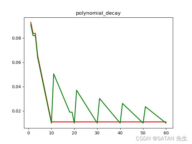
• 红线表示 cycle=False，当迭代次数超过 decay_steps 后，保持 end_learning_rate 不再改变；绿线表示 cycle=True，当迭代次数超过 decay_steps 后，学习率从 end_learning_rate 上升到一个数值后，再次执行衰减。
• 可以看到周期并没有变大。
• 多项式衰减中设置学习率可以往复升降的目的是为了防止神经网络后期训练的学习率过小，导致网络参数陷入某个局部最优解出不来，设置学习率升高机制，有可能使网络跳出局部最优解[1]。
• 上升的值是逐渐变小的，因为随着 $decay\_steps$ 逐渐变大，$\frac{global\_step}{decay\_steps}$ 趋向于 1，最后可能几乎没有上升。像不像一山更比一山矮？刚开始跳得远，最后跳得近。

4. natural_exp_decay(自然指数衰减)

tf.train.natural_exp_decay(
    learning_rate,  # 初始学习率
    global_step,
    decay_steps,    # 衰减速度，指数部分，越大衰减越慢
    decay_rate,     # 衰减速度，与 decay_steps 相反
    staircase=False,
    name=None
)

以 learning_rate 为初始值，学习率随 global_step 的增长呈自然指数衰减，衰减速度由 decay_steps 和 decay_rate（指数变化快慢）决定。公式：

$$current\_lr=learning\_rate\ast exp(-decay\_rate\ast \frac{global\_step}{decay\_steps})$$

参数 staircase 和 exponential_decay(指数衰减) 中的一样。

使用示例：

import matplotlib.pyplot as plt
import tensorflow as tf

global_step = tf.Variable(0, name='global_step', trainable=False)
learning_rate_1 = tf.train.natural_exp_decay(  # 阶梯型衰减
	learning_rate=0.6, global_step=global_step, decay_steps=10,
	decay_rate=0.6,
	staircase=True
)
learning_rate_2 = tf.train.natural_exp_decay(  # 步步衰减
	learning_rate=0.6, global_step=global_step, decay_steps=10,
	decay_rate=0.6,
	staircase=False
)
add1 = tf.assign_add(global_step, 1)

steps, lrs_1, lrs_2 = [], [], []
with tf.Session() as sess:
	sess.run(tf.global_variables_initializer())
	for _ in range(60):
		current_step, current_lr_1, current_lr_2, _ = sess.run([global_step, learning_rate_1, learning_rate_2, add1])
		steps.append(current_step)
		lrs_1.append(current_lr_1)
		lrs_2.append(current_lr_2)

plt.plot(steps, lrs_1, 'r-', linewidth=2)
plt.plot(steps, lrs_2, 'g-', linewidth=2)
plt.title('natural_exp_decay')
plt.show()

natural_exp_decay 学习率衰减

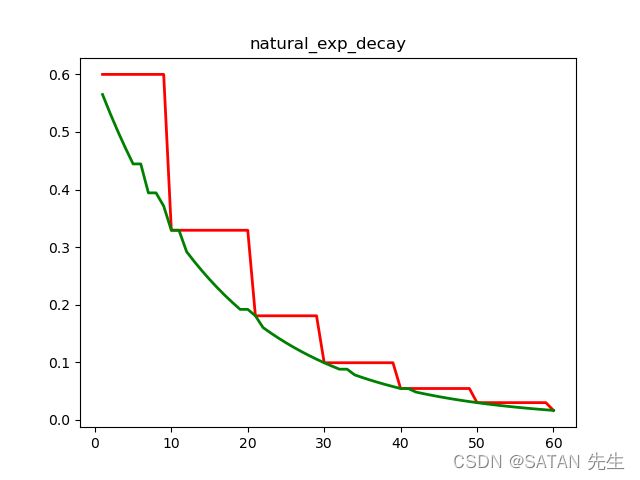
本质上和 exponential_decay 是一样的。我们看公式：

$$\begin{array}{rl}exponential\_lr& =learning\_rate\ast pow(decay\_rate,\frac{global\_step}{decay\_steps})\\ natural\_exp\_lr& =learning\_rate\ast exp(-decay\_rate\ast \frac{global\_step}{decay\_steps})\\ & =learning\_rate\ast pow(e^{-decay\_rate},\frac{global\_step}{decay\_steps})\end{array}$$

只要把 exponential_decay 中的 $decay\_rate$ 和 natural_exp_decay 中的 $e^{-decay\_rate}$ 设置成一样，那么两者就完全一样。

5. inverse_time_decay(倒数衰减)

tf.train.inverse_time_decay(
    learning_rate,  # 初始学习率
    global_step,
    decay_steps,    # 衰减快慢，越大衰减越慢
    decay_rate,     # 衰减快慢，越小衰减越慢
    staircase=False,# 与指数衰减相同
    name=None
)

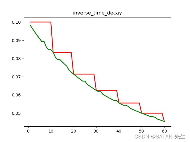
这跟指数衰减差不多，只不过把指数函数换成了倒数函数，可能下降得相对慢一点吧。公式：

$$current\_lr=learning\_rate/(1+decay\_rate\ast \frac{global\_step}{decay\_steps})$$

使用示例：

import matplotlib.pyplot as plt
import tensorflow as tf

global_step = tf.Variable(0, name='global_step', trainable=False)
learning_rate_1 = tf.train.inverse_time_decay(  # 阶梯型衰减
	learning_rate=0.1, global_step=global_step, decay_steps=10,
	decay_rate=0.2,
	staircase=True
)
learning_rate_2 = tf.train.inverse_time_decay(  # 步步衰减
	learning_rate=0.1, global_step=global_step, decay_steps=10,
	decay_rate=0.2,
	staircase=False
)
add1 = tf.assign_add(global_step, 1)

steps, lrs_1, lrs_2 = [], [], []
with tf.Session() as sess:
	sess.run(tf.global_variables_initializer())
	for _ in range(60):
		current_step, current_lr_1, current_lr_2, _ = sess.run([global_step, learning_rate_1, learning_rate_2, add1])
		steps.append(current_step)
		lrs_1.append(current_lr_1)
		lrs_2.append(current_lr_2)

plt.plot(steps, lrs_1, 'r-', linewidth=2)
plt.plot(steps, lrs_2, 'g-', linewidth=2)
plt.title('inverse_time_decay')
plt.show()

inverse_time_decay 学习率衰减

6. 各种余弦衰减

6.1 cosine_decay(余弦衰减)

tf.train.cosine_decay(
    learning_rate,  # 初始学习率
    global_step,
    decay_steps,    # 衰减步数，之后不再衰减
    alpha=0.0,      # learning_rate ∗ alpha 为最低学习率
    name=None
)

学习率呈余弦式衰减，前期缓慢衰减，中期快速，后期又缓慢，decay_steps 步后，衰减到最低学习率 learning_rate ∗ alpha 并保持。公式：

$$\begin{array}{rl}global\_step& =min(global\_step,decay\_steps)\\ cosine\_decay& =0.5\ast (1+cos(pi\ast \frac{global\_step}{decay\_steps}))\\ current\_lr& =learning\_rate\ast ((1-alpha)\ast cosine\_decay+alpha)\end{array}$$

在 $cosine\_decay$ 表达式中，$cos$ 部分随着 $global\_step$ 增加从 $cos(0)=1$ 逐渐降低到 $cos(pi)=-1$ 后保持不变，则 $cosine\_decay$ 从 1 沿余弦函数曲线下降到 0 后维持不变，最终 $current\_lr=learning\_rate\ast alpha$ [1]。

6.2 cosine_decay_restarts(重启式余弦衰减)

tf.train.cosine_decay_restarts(
    learning_rate,
	global_step,
	first_decay_steps,  # 第一个衰减期的衰减步数
	t_mul=2.0,          # 每次 restart，decay_steps 都会递归地乘以 t_mul
	m_mul=1.0,          # 每次 restart，learning_rate 都会递归地乘以 m_mul
	alpha=0.0,
	name=None
)

带重启的余弦式衰减，每个衰减期的过程都和 cosine_decay 一样。first_decay_steps 步后，衰减到最低学习率 learning_rate ∗ alpha，然后重启。新的衰减期中：learning_rate *= m_mul，decay_steps *= t_mul。如此反复。

6.3 linear_cosine_decay(线性余弦衰减)

tf.train.linear_cosine_decay(
    learning_rate,
    global_step,
    computation.
    decay_steps,
    num_periods=0.5,  # 衰减期内余弦函数的周期数（这类似重启但更加灵活）
    alpha=0.0,
    beta=0.001,  # 最小学习率为 learning_rate * beta
    name=None
)

同时进行线性衰减和余弦衰减的双重衰减，体现在两者相乘。公式：

$$\begin{array}{rl}global\_step& =min(global\_step,decay\_steps)\\ linear\_decay& =\frac{decay\_steps-global\_step}{decay\_steps}=1-\frac{global\_step}{decay\_steps}\\ cosine\_decay& =0.5\ast (1+cos(pi\ast 2\ast num\_periods\ast \frac{global\_step}{decay\_steps}))\\ current\_lr& =learning\_rate\ast ((alpha+linear\_decay)\ast cosine\_decay+beta)\\ & =learning\_rate\ast ((1+alpha-\frac{global\_step}{decay\_steps})\ast cosine\_decay+beta)\end{array}$$

相比 cosine_decay 增加了两个特性：

（1）与线性衰减相乘的效果为：后期相对前期衰减更快（线性衰减的叠加）；
（2）num_periods 可以灵活设置衰减期内余弦函数的周期数，默认是半个周期（余弦值从 1 到 0），若设置为默认值，则和 cosine_decay 相同。

6.4 noisy_linear_cosine_decay(噪声线性余弦衰减)

tf.train.noisy_linear_cosine_decay(
    learning_rate,
    global_step,
    decay_steps,
    initial_variance=1.0,  # initial variance for the noise. 
    variance_decay=0.55,   # decay for the noise's variance. See computation above.
    num_periods=0.5,       # Number of periods in the cosine part of the decay. 
    alpha=0.0,
    beta=0.001,
    name=None
)

相比 linear_cosine_decay，在线性部分加入了高斯扰动，具体有什么用咱也不清楚。$decayed$ 变为：

$$decayed=(alpha+linear\_decay+eps\_t)\ast cosine\_decay+beta$$

线性部分多了个 $eps\_t$，由 initial_variance 和 variance_decay 决定（暂不研究）。

6.5 对以上四种余弦衰减策略，画在同一张图中：

import matplotlib.pyplot as plt
import tensorflow as tf

global_step = tf.Variable(0, name='global_step', trainable=False)
learning_rate_1 = tf.train.cosine_decay(
	learning_rate=0.3, global_step=global_step, decay_steps=50,
	alpha=0.01
)
learning_rate_2 = tf.train.cosine_decay_restarts(
	learning_rate=0.3, global_step=global_step, first_decay_steps=10,
	t_mul=1.5,
	m_mul=0.8,
	alpha=0.011
)
learning_rate_3 = tf.train.linear_cosine_decay(
	learning_rate=0.3, global_step=global_step, decay_steps=50,
	num_periods=3.0,
	alpha=0.0,
	beta=0.2
)
learning_rate_4 = tf.train.noisy_linear_cosine_decay(
	learning_rate=0.1, global_step=global_step, decay_steps=50,
	initial_variance=0.01,
	variance_decay=0.1,
	num_periods=0.2,
	alpha=0.5,
	beta=0.2
)

add1 = tf.assign_add(global_step, 1)

steps, lrs_1, lrs_2, lrs_3, lrs_4 = [], [], [], [], []
with tf.Session() as sess:
	sess.run(tf.global_variables_initializer())
	for _ in range(60):
		current_step, current_lr_1, current_lr_2, current_lr_3, current_lr_4, _ = sess.run(
			[global_step, learning_rate_1, learning_rate_2, learning_rate_3, learning_rate_4, add1]
		)
		steps.append(current_step)
		lrs_1.append(current_lr_1)
		lrs_2.append(current_lr_2)
		lrs_3.append(current_lr_3)
		lrs_4.append(current_lr_4)

plt.plot(steps, lrs_1, 'r-', linewidth=2)
plt.plot(steps, lrs_2, 'g-', linewidth=2)
plt.plot(steps, lrs_3, 'b-', linewidth=2)
plt.plot(steps, lrs_4, 'y-', linewidth=2)
plt.title('cosine_decay')
plt.show()

inverse_time_decay 学习率衰减

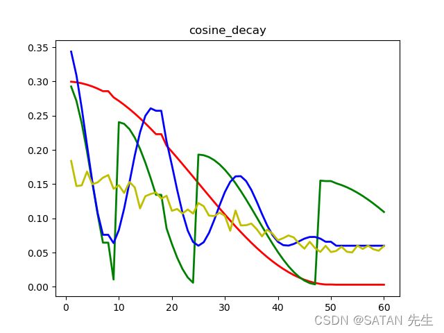
红色为标准余弦衰减（cosine_decay）；绿色为重启式余弦衰减（cosine_decay_restarts）；蓝色为线性余弦衰减（linear_cosine_decay）；黄色为噪声线性余弦衰减（noisy_linear_cosine_decay）;

看起来 linear_cosine_decay 比 cosine_decay_restarts 更加丝滑。

---

References

[1] 深度学习中常用的学习率衰减策略及tensorflow实现