雷达原理---线性调频信号的时频域分析

一、线性调频信号的时域分析

线性调频信号是通过非线性相位调制或线性频率调制获得大时宽带宽积的典型例子。

通常又把线性调频信号称为$chirp$信号。

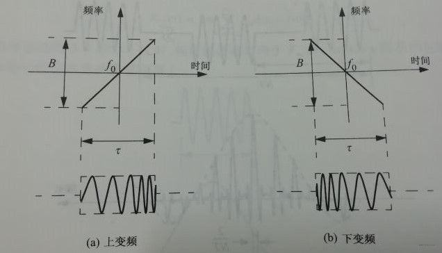
频率在脉宽内线性扫描，或者向上（上调频）或者向下（下调频）。

1. LFM上变频波形的瞬时相位可以表示为
   $$\phi (t)=2\pi (f_{0}t+\frac{\mu }{2}{t}^2)，-\frac{\tau }{2}\le t\le \frac{\tau }{2}$$
   其中，$f_0$为雷达中心频率，$\mu =\frac{B}{\tau }$为调频斜率，$\tau$为脉宽，$B$为带宽。因此，瞬时频率为
   $$f(t)=\frac{1}{2\pi }\frac{\mathrm{d}\phi (t)}{\mathrm{d}t}=f_0+\mu t，-\frac{\tau }{2}\le t\le \frac{\tau }{2}$$

2. 同理，下变频波形的瞬时相位和频率分别为
   $$\phi (t)=2\pi (f_{0}t-\frac{\mu }{2}{t}^2)，-\frac{\tau }{2}\le t\le \frac{\tau }{2}$$
   $$f(t)=\frac{1}{2\pi }\frac{\mathrm{d}\phi (t)}{\mathrm{d}t}=f_0-\mu t，-\frac{\tau }{2}\le t\le \frac{\tau }{2}$$
   

3. 典型的线性调频信号可以表示为

• 余弦形式

$$s(t)=rect(\frac{t}{\tau })cos(2\pi f_{0}t+\pi \mu t^2)$$

• 指数形式

$$s(t)=rect(\frac{t}{\tau })e^{j(2\pi f_{0}t+\pi \mu t^2)}$$
 其中，矩形调制函数$rect(\frac{t}{\tau })=\{\begin{array}{l}1，\left|\begin{array}{c}\frac{t}{\tau }\end{array}\right|\le \frac{\tau }{2}\\ 0，\left|\begin{array}{c}\frac{t}{\tau }\end{array}\right|>\frac{\tau }{2}\end{array}$

4. 线性调频信号的时宽带宽积$D$是一个重要参数，可以表示为
   $$D=\tau B=\mu {\tau }^2$$

二、线性调频信号的频域分析

1. 傅里叶变换

• 对$s(t)$进行傅里叶变换，
  $\begin{array}{rl}S(f)& ={\int }_{-\infty }^{\infty }s(t)e^{-j2\pi ft}dt\\ & ={\int }_{-\infty }^{\infty }rect(\frac{t}{T})e^{j(2\pi f_{0}t+\pi \mu t^2-2\pi ft)}dt\\ & ={\int }_{-\frac{T}{2}}^{\frac{T}{2}}{e}^{j\pi \mu t^2}{e}^{-j2\pi (f-f_0)t}dt\\ & ={\int }_{-\frac{T}{2}}^{\frac{T}{2}}{e}^{j\pi \mu [t^2-\frac{2(f-f_{0}t)}{\mu }]}dt\\ & ={\int }_{-\frac{T}{2}}^{\frac{T}{2}}{e}^{j\pi \mu [t^2-\frac{2(f-f_0)t}{\mu }+(\frac{f-f_0}{\mu }{)}^2]}{e}^{-j\pi \mu (\frac{f-f_0}{\mu }{)}^2}dt\\ & =e^{-j\pi \mu (\frac{f-f_0}{\mu }{)}^2}{\int }_{-\frac{T}{2}}^{\frac{T}{2}}{e}^{j\pi \mu [t-(\frac{f-f_0}{\mu }){]}^2}dt\\ & 令x=\sqrt{2\mu }(t-\frac{f-f_0}{\mu })\\ & =\frac{1}{\sqrt{2\mu }}{e}^{-j\pi \mu (\frac{f-f_0}{\mu }{)}^2}{\int }_{\sqrt{2\mu }(-\frac{T}{2}-\frac{f-f_0}{\mu })}^{\sqrt{2\mu }(\frac{T}{2}-\frac{f-f_0}{\mu })}{e}^{j\frac{\pi }{2}{x}^2}dx\\ & 不妨设{\mu }_1=\sqrt{2\mu }(\frac{T}{2}-\frac{f-f_0}{\mu })，{\mu }_2=\sqrt{2\mu }(\frac{T}{2}+\frac{f-f_0}{\mu })\\ & =\frac{1}{\sqrt{2\mu }}{e}^{-j\pi \mu (\frac{f-f_0}{\mu }{)}^2}{\int }_{-{\mu }_2}^{{\mu }_1}{e}^{j\frac{\pi }{2}{x}^2}dx\\ & =\frac{1}{\sqrt{2\mu }}{e}^{-j\pi \mu (\frac{f-f_0}{\mu }{)}^2}({\int }_{-{\mu }_2}^{{\mu }_1}cos\frac{\pi }{2}{x}^{2}dx+j{\int }_{-{\mu }_2}^{{\mu }_1}sin\frac{\pi }{2}{x}^{2}dx)\\ & =\frac{1}{\sqrt{2\mu }}{e}^{-j\pi \mu (\frac{f-f_0}{\mu }{)}^2}({\int }_{-{\mu }_2}^{0}cos\frac{\pi }{2}{x}^{2}dx+{\int }_0^{{\mu }_1}cos\frac{\pi }{2}{x}^{2}dx+j{\int }_{-{\mu }_2}^{0}sin\frac{\pi }{2}{x}^{2}dx+j{\int }_0^{{\mu }_1}sin\frac{\pi }{2}{x}^{2}dx)\\ & =\frac{1}{\sqrt{2\mu }}{e}^{-j\pi \mu (\frac{f-f_0}{\mu }{)}^2}(-{\int }_0^{-{\mu }_2}cos\frac{\pi }{2}{x}^{2}dx+{\int }_0^{{\mu }_1}cos\frac{\pi }{2}{x}^{2}dx-j{\int }_0^{-{\mu }_2}sin\frac{\pi }{2}{x}^{2}dx+j{\int }_0^{{\mu }_1}sin\frac{\pi }{2}{x}^{2}dx)\\ & =\frac{1}{\sqrt{2\mu }}{e}^{-j\pi \mu (\frac{f-f_0}{\mu }{)}^2}\left(\right[C({\mu }_2)+C({\mu }_1)]+j[S({\mu }_2)+S({\mu }_1)\left]\right)\end{array}$

• 那么其幅度谱可表示为$$\left|S(f)\right|=\frac{1}{\sqrt{2\mu }}\left(\right[C({\mu }_2)+C({\mu }_1){]}^2+[S({\mu }_2)+S({\mu }_1){]}^2{)}^{\frac{1}{2}}$$
  相位谱可表示为$$\phi (f)=-\frac{\pi }{\mu }(f-f_0{)}^2+arctan\frac{S({\mu }_2)+S({\mu }_1)}{C({\mu }_2)+C({\mu }_1)}$$

• 其中，$C(x)$和$S(x)$表示菲涅耳积分，定义如下：
  $$C(x)={\int }_0^{x}cos(\frac{\pi {\xi }^2}{2})d\xi$$
  $$S(x)={\int }_0^{x}sin(\frac{\pi {\xi }^2}{2})d\xi$$
  菲涅尔积分近似为
  $$C(x)\approx \frac{1}{2}+\frac{1}{\pi x}sin(\frac{\pi }{2}{x}^2)，x\gg 1$$
  $$S(x)\approx \frac{1}{2}-\frac{1}{\pi x}cos(\frac{\pi }{2}{x}^2)，x\gg 1$$
  并且$C(-x)=-C(x)，S(-x)=-S(x)$

• 当时宽带宽积足够大时，$C(\mu )=S(\mu )=\sqrt{\frac{\pi }{8}}$

 即$$\begin{array}{rl}\left|S(f)\right|& =\sqrt{\frac{\pi }{2\mu }}rect(\frac{f}{B})\\ \phi (f)& =-\frac{\pi }{\mu }(f-f_0{)}^2+\frac{\pi }{4}\end{array}$$

2. 驻定相位原理（Principle of Stationary Phase，PSP）

2.1 作用：

一种求解复杂高频扰动信号的近似积分方法；适用于相位包含二次及高次项且包络缓变的信号频谱求解。

2.2 原理：

在驻相点附近，信号的相位变化非常小，相位值有很长时间的滞留，对积分的贡献能够得以显现；而其他位置，相位变化非常大，积分近似为零。

2.3 一般式推导：

以通用信号（高频扰动信号）$x(t)=A(t)e^{j\theta (t)}$的傅里叶变换，推导驻相原理。
$$X(w)={\int }_{-\infty }^{\infty }A(t)e^{j\theta (t)}{e}^{-jwt}dt={\int }_{-\infty }^{\infty }A(t)e^{j[\theta (t)-wt]}dt={\int }_{-\infty }^{\infty }A(t)e^{j\phi (t,w)}dt$$
其中，令$\phi (t)=\theta (t)-wt；$

根据PSP，积分在$\frac{d\phi (t)}{dt}=0$附近才显著地不为零；令${\phi }^{{}^{\prime }}(t){|}_{t=t_s}=0$所得$t_s$即为驻相点。

在驻定相位点处对$\phi (t)$进行泰勒展开：
$$\phi (t)=\phi (t_s)+{\phi }^{{}^{\prime }}(t_s)(t-t_s)+\frac{1}{2}{\phi }^{{}^{\prime \prime }}(t_s)(t-t_s{)}^2+\dots \dots$$
忽略高次项，则
$$\phi (t)=\phi (t_s)+\frac{1}{2}{\phi }^{{}^{\prime \prime }}(t_s)(t-t_s{)}^2$$
代入信号频域表达式
$$X(f)={\int }_{-\infty }^{\infty }A(t_s)e^{j\phi (t)}dt=A(t_s)e^{j\phi (t_s)}{\int }_{-\infty }^{\infty }{e}^{j\frac{{\phi }^{{}^{\prime \prime }}(t_s)}{2}(t-t_s{)}^2}dt=A(t_s)e^{j\phi (t_s)}{\int }_{t_s-\delta }^{t_s+\delta }{e}^{j\frac{{\phi }^{{}^{\prime \prime }}(t_s)}{2}(t-t_s{)}^2}dt$$
作变量代换

$$t-t_s=u及\frac{{\phi }^{{}^{\prime \prime }}(t_s)}{2}{u}^2=\frac{\pi y^2}{2}$$
则$$du=\sqrt{\frac{\pi }{{\phi }^{{}^{\prime \prime }}(t_s)}}dy$$

代入信号频域表达式
$$X(f)=2\sqrt{\pi }\frac{A(t_s)}{\sqrt{{\phi }^{{}^{\prime \prime }}(t_s)}}{e}^{j\phi (t_s)}{\int }_0^{\sqrt{\frac{{\phi }^{{}^{\prime \prime }}(t_s)}{\pi }}\delta }{e}^{j\frac{\pi y^2}{2}}dy$$

若积分上限较大，则菲涅尔积分趋于
$${\int }_0^{\infty }{e}^{j\frac{\pi y^2}{2}}dy=\sqrt{\frac{\pi }{8}}\sqrt{\frac{2}{\pi }}(1+j)=\frac{1}{\sqrt{2}}{e}^{j\frac{\pi }{4}}$$

由此，上述傅里叶变换的积分近似解为
$$X(f)\approx \sqrt{\frac{2\pi }{{\phi }^{{}^{\prime \prime }}(t_s)}}A(t_s)e^{j\phi (t_s)}{e}^{j\frac{\pi }{4}}$$

2.4 LFM频域表达式近似解

$$s(t)=rect(\frac{t}{T})e^{j\pi K{t}^2}$$
可得$$S(f)=\frac{1}{\sqrt{K}}rect(\frac{f}{KT})e^{-j\pi \frac{f^2}{K}}{e}^{j\frac{\pi }{4}}$$

三、MATLAB仿真

1、菲涅尔积分

• 代码：

syms x;
fplot(fresnelc(x),[-4 4]);
hold on;
grid on;
fplot(fresnels(x),[-4 4],'--');
xlabel('x');
ylabel('Fresnel integrals:C(x)，S(x)');
legend('C(x)','S(x)');

• 结果：
  

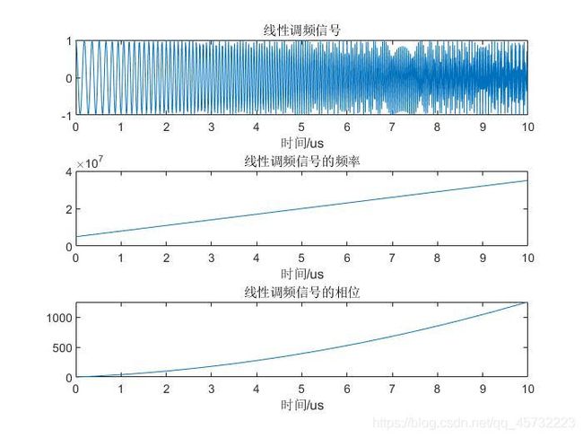
2、线性调频信号

• 代码：

clear all;
close all;
clc;
%%%%%%%%%%线性调频信号的时域分析%%%%%%%%%%
TimeWidth=10e-6;       %信号时宽
BandWidth=30e6;        %信号带宽
Fs=80e6;               %采样频率，个人理解：根据奈奎斯特采样定理，要求采样频率大于2倍的信号最高频率，而对于线性调频信号信号最高频率为F0+B
F0=5e6;                %中频频率

N=fix(TimeWidth*Fs);                      %采样点数，fix函数向零方向取整
FFT_Len=2^nextpow2(N);                    %计算FFT的长度：为了提高FFT算法的性能，要求信号长度为2的幂
t=(0:N-1)/Fs;

st=cos(2*pi*F0*t+pi*(BandWidth/TimeWidth)*t.^2);  %线性调频信号余弦表达式
figure;
subplot(3,1,1);
plot(t*1e6,st);
xlabel('时间/us');
title('线性调频信号');

f=F0+(BandWidth/TimeWidth)*t;
subplot(3,1,2);
plot(t*1e6,f);
xlabel('时间/us');
title('线性调频信号的频率');

phase=2*pi*F0*t+pi*(BandWidth/TimeWidth)*t.^2;
subplot(3,1,3);
plot(t*1e6,phase);
xlabel('时间/us');
title('线性调频信号的相位');

%%%%%%%%%%线性调频信号的频域分析%%%%%%%%%%
fs=(0:FFT_Len-1)*Fs/FFT_Len;
Sf=(fftshift(fft(st,FFT_Len)));
figure;
plot(fs*1e-6,abs(Sf));
xlabel('频率/MHz');
title('线性调频信号的幅度谱');

• 结果：