SparkMLib决策树和逻辑斯蒂回归的示例

SparkMLib 编程基础

实验目的：

• 通过实验掌握Spark MLlib 的基本编程方法；
• 熟悉spark与数据挖掘和机器学习的综合使用；

实验内容：
数据从美国 1994 年人口普查数据 库抽取而来，可用来预测居民收入是否超过 50K$/year。该数据集类变量为年收入是否超过50k$，属性变量包含年龄、工种、学历、职业、人种等重要信息，值得一提的是，14 个属 性变量中有 7 个标签变量。

#step0.环境准备

from pyspark import SparkConf, SparkContext
from pyspark.sql import SparkSession

spark = SparkSession.builder.master('local[6]').appName('spark-ml').getOrCreate()
spark.sparkContext.setLogLevel('WARN')

#step1.从文件中导入数据adult.data.txt和测试数据adult.test.txt，并转化为 DataFrame

from pyspark.sql.types import *

# 设置schema
schema = StructType([
    StructField('age', IntegerType()),
    StructField('workclass', StringType()),
    StructField('fnlwgt', IntegerType()),
    StructField('education', StringType()),
    StructField('educationNum', IntegerType()),
    StructField('maritalStatus', StringType()),
    StructField('occupation', StringType()),
    StructField('relationship', StringType()),
    StructField('race', StringType()),
    StructField('sex', StringType()),
    StructField('capitalGain', IntegerType()),
    StructField('capitalLoss', IntegerType()),
    StructField('hoursPerWeek', IntegerType()),
    StructField('nativeCountry', StringType()),
    StructField('50K', StringType())
])

adult_data_path = 'file:///home/chenE2000/code/pyspark/data/adult.data.csv'
adult_test_path = 'file:///home/chenE2000/code/pyspark/data/adult.test.csv'

# 读入rdd
adult_data = spark.read.csv(adult_data_path, header=False, schema=schema, ignoreLeadingWhiteSpace=True)
adult_test = spark.read.csv(adult_test_path, header=False, schema=schema, ignoreLeadingWhiteSpace=True)

不要忘记ignoreLeadingWhiteSpace参数 它可以有效地去除数据之前的空格

#step2.进行主成分分析（PCA）

对6个连续型的数值型变量进行主成分分析。PCA（主成分分析）是通过正交变换把一 组相关变量的观测值转化成一组线性无关的变量值，即主成分的一种方法。PCA 通过使用 主成分把特征向量投影到低维空间，实现对特征向量的降维。请通过setK()方法将主成分数 量设置为3，把连续型的特征向量转化成一个3维的主成分。

分析：

如下的features为连续值：

age fnlwgt educationNum capitalGain capitalLoss hoursPerWeek

from pyspark.ml.feature import PCA
from pyspark.ml.feature import VectorAssembler

# 选择需要进行分析的features
pca_features = ['age', 'fnlwgt', 'educationNum', 'capitalGain', 'capitalLoss', 'hoursPerWeek']

# 创建VectorAssembler
vecAssembler = VectorAssembler(inputCols=pca_features, outputCol="features")
df = adult_data.select(pca_features)

# 对df进行VectorAssembler的transform
converted_df = vecAssembler.transform(df)
# converted_df.show()

# 初始化PCA对象
pca = PCA(k=3, inputCol="features", outputCol="pca_features")
# 对converted_df中的features进行PCA
model = pca.fit(converted_df)
model.transform(converted_df).select('features' ,'pca_features').show(5)

OUTPUT
+--------------------+--------------------+
|            features|        pca_features|
+--------------------+--------------------+
|[39.0,77516.0,13....|[77516.0654328193...|
|[50.0,83311.0,13....|[83310.9993559577...|
|[38.0,215646.0,9....|[215645.999250486...|
|[53.0,234721.0,7....|[234720.999079618...|
|[28.0,338409.0,13...|[338408.999188305...|
+--------------------+--------------------+
only showing top 5 rows

#step3.训练分类模型并预测居民收入

任务： 在主成分分析的基础上，采用逻辑斯蒂回归，或者决策树模型预测居民收入是否超过 50K；对测试数据集进行验证。

有能力的情况下可以在此处进行数据清洗，以达到更佳的性能！

# 对非连续的features进行特征工程
from pyspark.ml.feature import StringIndexer

categorical_features = ['workclass', 'education', 'maritalStatus', 'occupation', 'relationship', 'race', 'sex', 'nativeCountry', '50K']

def categorical_transform(data):
    categorical_transformed = data
    # 该版本不支持inputCols和outputCols 只得一列一列来
    for feature in categorical_features:
        indexer = StringIndexer(inputCol=feature, outputCol='{}Index'.format(feature))
        model = indexer.fit(categorical_transformed)
        categorical_transformed = model.transform(categorical_transformed)

    return categorical_transformed

# 提取特征features
continues_features = ['age', 'fnlwgt', 'educationNum', 'capitalGain', 'capitalLoss', 'hoursPerWeek']
categorical_indexed_features = ['{}Index'.format(x) for x in categorical_features[:-1]]

features = continues_features + categorical_indexed_features

# 创建VectorAssembler
vecAssembler = VectorAssembler(inputCols=features, outputCol="features")

# 对df进行VectorAssembler的transform
trainDf = vecAssembler.transform(categorical_transform(adult_data))
testDf = vecAssembler.transform(categorical_transform(adult_test))

- 决策树

from pyspark.ml.classification import DecisionTreeClassifier
from pyspark.ml.evaluation import MulticlassClassificationEvaluator
import matplotlib.pyplot as plt

evaluator = MulticlassClassificationEvaluator(predictionCol='prediction', labelCol='50KIndex')

# 创建决策树模型 输入训练数据
def train(trainDf, maxDepth):
    DTC = DecisionTreeClassifier(featuresCol='features', labelCol='50KIndex', maxBins=42, maxDepth=maxDepth)
    DTM = DTC.fit(trainDf)

    # 获取训练数据和测试数据结果
    modelDF = DTM.transform(trainDf)
    testPrediction = DTM.transform(testDf)

    # 验证决策树
    return ((maxDepth, evaluator.evaluate(modelDF), evaluator.evaluate(testPrediction)))

def analysis():
    acc = []
    for maxDepth in range(1, 20):
        res = train(trainDf, maxDepth)
        acc.append(res)
        print('maxDepth:', res[0], 'train accuracy:', res[1], 'test accuracy:', res[2])

    # 绘制图形
    maxDepths = list(map(lambda x: x[0], acc))
    trainAccuracys = list(map(lambda x: x[1], acc))
    testAccuracys = list(map(lambda x: x[2], acc))
    plt.plot(maxDepths, trainAccuracys, c='b')
    plt.plot(maxDepths, testAccuracys, c='r')

analysis()

OUTPUT
maxDepth: 1 train accuracy: 0.6552674618087769 test accuracy: 0.6614797504945593
maxDepth: 2 train accuracy: 0.8109320624905785 test accuracy: 0.8133628331723791
maxDepth: 3 train accuracy: 0.8310154235710148 test accuracy: 0.8316567148818761
maxDepth: 4 train accuracy: 0.8313485776444282 test accuracy: 0.832020522874436
maxDepth: 5 train accuracy: 0.8369674407658547 test accuracy: 0.8146261911749816
maxDepth: 6 train accuracy: 0.843850231385477 test accuracy: 0.8417373266949746
maxDepth: 7 train accuracy: 0.8465528793663664 test accuracy: 0.8409960462809405
maxDepth: 8 train accuracy: 0.8508643825697595 test accuracy: 0.8399204152510952
maxDepth: 9 train accuracy: 0.8620958061438972 test accuracy: 0.846430906055735
maxDepth: 10 train accuracy: 0.8666366083784642 test accuracy: 0.8475413915197532
maxDepth: 11 train accuracy: 0.8717244675803354 test accuracy: 0.8414804546022179
maxDepth: 12 train accuracy: 0.8776113185658438 test accuracy: 0.8407129903622617
maxDepth: 13 train accuracy: 0.8846079071716166 test accuracy: 0.8366190631184339
maxDepth: 14 train accuracy: 0.8914897265340832 test accuracy: 0.8337211492420662
maxDepth: 15 train accuracy: 0.9000707429424302 test accuracy: 0.8278867396186974
maxDepth: 16 train accuracy: 0.9082849628562478 test accuracy: 0.8225457516098253
maxDepth: 17 train accuracy: 0.9167414880539138 test accuracy: 0.8144349145794498
maxDepth: 18 train accuracy: 0.926592822424274 test accuracy: 0.8133443581969498
maxDepth: 19 train accuracy: 0.934405490949558 test accuracy: 0.8113092125950603

看图发现：随着训练精度（蓝线）的不断提高，测试精度在maxDepth=9时达到最大值，随后波动下降，可以推断学习进入了过拟合。

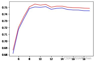
- 逻辑斯蒂回归（加入PCA）

from pyspark.ml.classification import LogisticRegression
from pyspark.ml.evaluation import MulticlassClassificationEvaluator
import matplotlib.pyplot as plt

evaluator = MulticlassClassificationEvaluator(predictionCol='prediction', labelCol='50KIndex')

# 创建决策树模型 输入训练数据
def evaluate(train, test, maxIter):
    LR = LogisticRegression(featuresCol='pca_features', labelCol='50KIndex', maxIter=maxIter, threshold=0.7)
    LRM = LR.fit(train)

    # 获取训练数据和测试数据结果
    modelDF = LRM.transform(train)
    testPrediction = LRM.transform(test)

    # 验证决策树
    return ((maxIter, evaluator.evaluate(modelDF), evaluator.evaluate(testPrediction)))

def analysis():
    # 对特征进行PCA k=5
    pca = PCA(k=5, inputCol="features", outputCol="pca_features")
    model = pca.fit(trainDf)
    train = model.transform(trainDf)
    model = pca.fit(testDf)
    test = model.transform(testDf)

    acc = []
    for maxIter in range(5, 20, 1):
        res = evaluate(train, test, maxIter)
        acc.append(res)
        print('maxIter:', res[0], 'train accuracy:', res[1], 'test accuracy:', res[2])

    # 绘制图形
    maxIter = list(map(lambda x: x[0], acc))
    trainAccuracys = list(map(lambda x: x[1], acc))
    testAccuracys = list(map(lambda x: x[2], acc))
    plt.plot(maxIter, trainAccuracys, c='b')
    plt.plot(maxIter, testAccuracys, c='r')

analysis()

OUTPUT
maxIter: 5 train accuracy: 0.6817131758963453 test accuracy: 0.6866887555058971
maxIter: 6 train accuracy: 0.7172453962565405 test accuracy: 0.7203214149689302
maxIter: 7 train accuracy: 0.7332999698583238 test accuracy: 0.7366913085364823
maxIter: 8 train accuracy: 0.7482561525095872 test accuracy: 0.7507269297293476
maxIter: 9 train accuracy: 0.7505142334457181 test accuracy: 0.7547939216709018
maxIter: 10 train accuracy: 0.7499930157195169 test accuracy: 0.7532343435490358
maxIter: 11 train accuracy: 0.750966562427745 test accuracy: 0.7542565770322758
maxIter: 12 train accuracy: 0.7470295056375074 test accuracy: 0.7501809696613664
maxIter: 13 train accuracy: 0.7485632057470427 test accuracy: 0.7516924341816431
maxIter: 14 train accuracy: 0.7489594896261998 test accuracy: 0.751683364879325
maxIter: 15 train accuracy: 0.7466916066862874 test accuracy: 0.7500588309038333
maxIter: 16 train accuracy: 0.746064839164776 test accuracy: 0.7494438122823357
maxIter: 17 train accuracy: 0.7459567085467473 test accuracy: 0.749351862343532
maxIter: 18 train accuracy: 0.7449322230371984 test accuracy: 0.7487953782757679
maxIter: 19 train accuracy: 0.7448465591356768 test accuracy: 0.748610137147232

小结

本次实验简单地体验了spark mlib工具包，对数据进行了简单的特征处理和模型调优。

在本次案例上，决策树的表现要优于LogisticRegression。

未来可以尝试对数据进行清洗与更加多的特征变换（归一化，主成分分析等）。