声纹识别中pooling总结
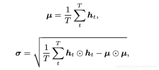
1、Statistics Pooling
http://danielpovey.com/files/2017_interspeech_embeddings.pdf
The statistics pooling layer calculates the mean vector µ as well as the second-order statistics as the standard deviation vector σ over frame-level features ht (t = 1, · · · , T ).
where ⊙ represents the Hadamard product.
2、Attentive Statistics Pooling
https://arxiv.org/pdf/1803.10963.pdf
calculates a scalar score et for each frame-level feature.
where f(·) is a non-linear activation function, such as a tanh or ReLU function.
The score is normalized over all frames by a softmax function so as to add up to the following unity:
The normalized score αt is then used as the weight in the pooling layer to calculate the weighted mean vector
the weighted standard deviation is defined as follows:
3、Self-Attentive pooling
https://danielpovey.com/files/2018_interspeech_xvector_attention.pdf
H = {h1, h2, · · · , hT }, where ht is the hidden representation of input frame xt captured by the hidden layer below the self-attention layer.
where W1 is a matrix of size dh × da; W2 is a matrix of size da × dr, and dr is a hyperparameter that represents the number of attention heads; g(·) is some activation function and ReLU is chosen here. The sof tmax(·) is performed column-wise.
Each column vector of A is an annotation vector that represents the weights for different ht. Finally the weighted means E is obtained by
By increasing dr, we can easily have multiple attention heads to learn different aspects from a speaker’s speech. To encourage diversity in the annotation vectors so that each attention head can extract dissimilar information from the same speech segment, a penalty term P is introduced when dr > 1:
where I is the identity matrix and k·kF represents the Frobenius norm of a matrix. P is similar to L2 regularization and is minimized together with the original cost of the whole system
4、self Multi-Head Attention pooling
https://ieeexplore.ieee.org/document/9053217
where Ti 1 is a temperature hyperparameter
5、NetVLAD
https://arxiv.org/pdf/1902.10107.pdf
https://arxiv.org/pdf/1511.07247.pdf
更详细的解释参考:https://zhuanlan.zhihu.com/p/96718053
6 learnable dictionary encoding (LDE)
https://arxiv.org/pdf/1804.05160.pdf
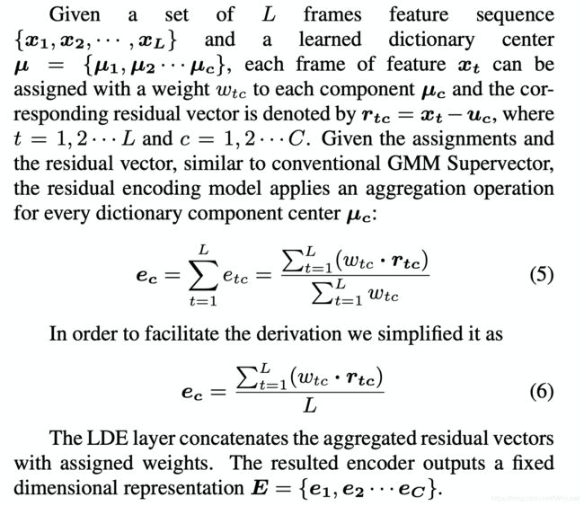
Here, we introduce two groups of learnable parameters. One is the dictionary component center, noted as µ = {µ1, µ2 · · · µc}. The other one is assigned weights, noted as w.
where the smoothing factor ![]() for each dictionary center
for each dictionary center ![]() is learnable.
is learnable.
7、Attentive bilinear pooling (ABP)
https://www.isca-speech.org/archive/Interspeech_2020/pdfs/1922.pdf
Specifically, let H ∈ RL×D be the frame-level feature map captured by the hidden layer below the self-attention layer, where L and D are the number of frames and feature dimension respectively. Then the attention map A ∈ RL×K can be obtained by feeding H into a 1×1 convolutional layer followed by softmax non-linear activation, where K is the number of attention heads. The 1 st-order and 2 nd-order attentive statistics of H, denoted by µ and σ 2 , can be computed similar as crosslayer bilinear pooling [4], which is
where T1(x) is the operation of reshaping x into a vector, and T2(x) includes a signed square-root step and a L2- normalization step. represents the Hadamard product. The output of ABP is the concatenation of µ and σ 2
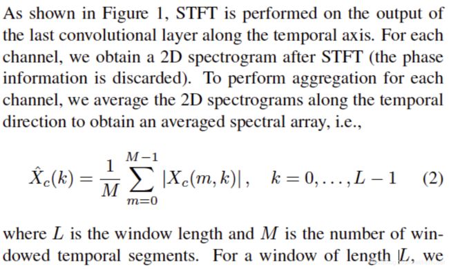
8、Short-time Spectral Pooling (STSP)
https://ieeexplore.ieee.org/stamp/stamp.jsp?tp=&arnumber=9414094
(完)


