机器学习之梯度与梯度下降法
寻找最佳模型的最优化问题的解决方案(Solution to sort of Optimization Problem to find the Best Model)
Frequently when doing data science, we’ll be trying to the find the best model for a certain situation. And usually “best” will mean something like “minimizes the error of the model” or “maximizes the likelihood of the data.” In other words, it will represent the solution to some sort of optimization problem.
在进行数据科学时,我们经常会尝试为特定情况找到最佳模型。 通常,“最佳”的意思是“使模型的误差最小化”或“使数据的可能性最大化”。 换句话说,它将代表某种优化问题的解决方案。
This means we’ll need to solve a number of optimization problems. And in particular, we’ll need to solve them from scratch. Our approach will be a technique called gradient descent, which lends itself pretty well to a from-scratch treatment. You might not find it super exciting in and of itself, but it will enable us to do exciting things throughout the article, so bear with me.
这意味着我们需要解决许多优化问题。 特别是,我们需要从头开始解决它们。 我们的方法是称为梯度下降的技术,该技术非常适合从头开始处理。 您可能并不觉得它本身超级有趣,但是它将使我们能够在整篇文章中做令人兴奋的事情,所以请耐心等待。
梯度下降背后的想法 (The Idea Behind Gradient Descent)
Suppose we have some function f that takes as input a vector of real numbers and outputs a single real number. One simple such function is:
假设我们有一些函数f,它接受一个实数向量作为输入并输出一个实数。 一种简单的此类功能是:
We’ll frequently need to maximize (or minimize) such functions. That is, we need to find the input “v” that produces the largest (or smallest) possible value.
我们经常需要最大化(或最小化)此类功能。 也就是说,我们需要找到产生最大(或最小)可能值的输入“ v”。
For functions like ours, the gradient (if you remember your calculus, this is the vector of partial derivatives) gives the input direction in which the function most quickly increases. (If you don’t remember your calculus, take my word for it or look it up on the Internet.)
对于像我们这样的函数,梯度(如果您还记得微积分,这就是偏导数的向量)给出函数最快速增加的输入方向。 (如果您不记得自己的演算,请相信我或在互联网上查找。)
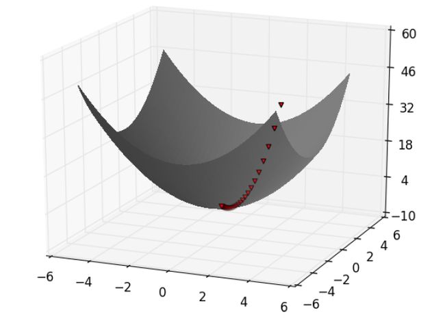
Accordingly, one approach to maximizing a function is to pick a random starting point, compute the gradient, take a small step in the direction of the gradient (i.e., the direction that causes the function to increase the most), and repeat with the new starting point. Similarly, you can try to minimize a function by taking small steps in the opposite direction.
因此,使函数最大化的一种方法是选择一个随机的起点,计算梯度,在梯度的方向(即导致函数增加最大的方向)上走一小步,然后用新的初始点。 同样,您可以尝试通过在相反方向上采取一些小步骤来最小化功能。
Finding a minimum using gradient descent 使用梯度下降找到最小值估计梯度(Estimating the Gradient)
If “f” is a function of one variable, its derivative at a point “x” measures how f(x) changes when we make a very small change to “x”. It is defined as the limit of the difference quotients:
如果“ f”是一个变量的函数,则当我们对“ x”进行很小的更改时,其在“ x”点的导数将测量f(x)的变化。 定义为差商的限制:
as “h” approaches zero.
当“ h”接近零时。
(Many a would-be calculus student has been stymied by the mathematical definition of limit. Here we’ll cheat and simply say that it means what you think it means.)
(许多想做微积分的学生已经被极限的数学定义所困扰。在这里,我们作弊并简单地说,这意味着您所认为的含义。)
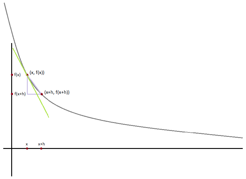
Approximating a derivative with a difference quotient 用差商近似导数The derivative is the slope of the tangent line at (x, f( x)), while the difference quotient is the slope of the not-quite-tangent line that runs through (x+h, f(x+h)). As “h” gets smaller and smaller, the not-quite-tangent line gets closer and closer to the tangent line.
导数是(x,f(x))处切线的斜率,而差商是穿过(x + h,f(x + h))的非切线的斜率。 随着“ h”变得越来越小,非正切线越来越接近切线。
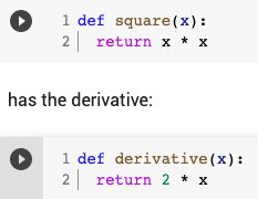
For many functions it’s easy to exactly calculate derivatives. For example, the square function:
对于许多函数来说,精确计算导数很容易。 例如,平方函数:
which you can check — if you are so inclined — by explicitly computing the difference quotient and taking the limit.
您可以通过显式计算差商并采用极限来检查(如果您愿意)。
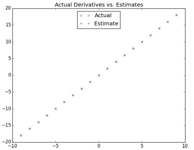
What if you couldn’t (or didn’t want to) find the gradient? Although we can’t take limits in Python, we can estimate derivatives by evaluating the difference quotient for a very small “e”.
如果您无法(或不想)找到渐变怎么办? 尽管我们无法在Python中使用限制,但可以通过评估很小的“ e”的差商来估计导数。
When “f” is a function of many variables, it has multiple partial derivatives, each indicating how “f” changes when we make small changes in just one of the input variables.
当“ f”是许多变量的函数时,它具有多个偏导数,每个偏导数表示当我们仅对输入变量之一进行细微更改时,“ f”如何变化。
We calculate its “ith” partial derivative by treating it as a function of just its ith variable, holding the other variables fixed:
通过将其视为第i个变量的函数,并固定其他变量,来计算其“第i个”偏导数:
after which we can estimate the gradient the same way:
之后我们可以用相同的方式估算梯度:
使用渐变 (Using the Gradient)
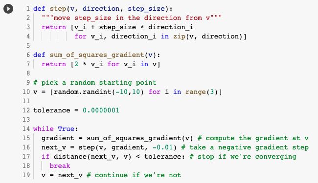
It’s easy to see that the sum_of_squares function is smallest when its input “v” is a vector of zeroes. But imagine we didn’t know that. Let’s use gradients to find the minimum among all three-dimensional vectors. We’ll just pick a random starting point and then take tiny steps in the opposite direction of the gradient until we reach a point where the gradient is very small:
很容易看出,当sum_of_squares函数的输入“ v”是零向量时,它最小。 但是想象一下我们不知道。 让我们使用梯度来查找所有三维向量中的最小值。 我们将选择一个随机的起点,然后在渐变的相反方向上执行一些小步骤,直到到达渐变很小的点:
If you run this, you’ll find that it always ends up with a “v” that’s very close to [0,0,0]. The smaller you make the tolerance, the closer it will get.
如果运行此命令,您会发现它始终以非常接近[0,0,0]的“ v”结尾。 公差越小,公差就越大。
选择正确的步长 (Choosing the Right Step Size)
Although the rationale for moving against the gradient is clear, how far to move is not. Indeed, choosing the right step size is more of an art than a science. Popular options include:
尽管逆梯度移动的原理很明确,但移动的距离尚不清楚。 的确,选择合适的步长是一门艺术,而不是一门科学。 热门选项包括:
• Using a fixed step size
•使用固定的步长
• Gradually shrinking the step size over time
•随着时间的推移逐步缩小步长
• At each step, choosing the step size that minimizes the value of the objective function
•在每个步骤中,选择最小化目标函数值的步长
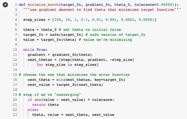
The last sounds optimal but is, in practice, a costly computation. We can approximate it by trying a variety of step sizes and choosing the one that results in the smallest value of the objective function:
最后一个听起来不错,但实际上却是一个昂贵的计算。 我们可以通过尝试各种步长并选择导致目标函数最小值的步长来近似估算:
It is possible that certain step sizes will result in invalid inputs for our function. So we’ll need to create a “safe apply” function that returns infinity (which should never be the minimum of anything) for invalid inputs:
某些步长可能会导致我们的功能输入无效。 因此,我们需要创建一个“安全应用”函数,为无效输入返回无穷大(永远不应为最小):
放在一起 (Putting It All Together)
In the general case, we have some target_fn that we want to minimize, and we also have its gradient_fn. For example, the target_fn could represent the errors in a model as a function of its parameters, and we might want to find the parameters that make the errors as small as possible.
在一般情况下,我们有一些要最小化的target_fn,也有它的gradient_fn。 例如,target_fn可以将模型中的错误表示为其参数的函数,我们可能希望找到使错误尽可能小的参数。
Furthermore, let’s say we have (somehow) chosen a starting value for the parameters theta_0. Then we can implement gradient descent as:
此外,假设我们(以某种方式)为参数theta_0选择了一个起始值。 然后我们可以将梯度下降实现为:
We called it minimize_batch because, for each gradient step, it looks at the entire data set (because target_fn returns the error on the whole data set). In the next section, we’ll see an alternative approach that only looks at one data point at a time.
我们之所以称它为“ minimum_batch”是因为,对于每个梯度步骤,它都会查看整个数据集(因为target_fn返回整个数据集的错误)。 在下一节中,我们将看到另一种方法,一次仅查看一个数据点。
Sometimes we’ll instead want to maximize a function, which we can do by minimizing its negative (which has a corresponding negative gradient):
有时我们想最大化一个函数,可以通过最小化其负数(具有相应的负梯度)来实现:
随机梯度下降 (Stochastic Gradient Descent)
As we mentioned before, often we’ll be using gradient descent to choose the parameters of a model in a way that minimizes some notion of error. Using the previous batch approach, each gradient step requires us to make a prediction and compute the gradient for the whole data set, which makes each step take a long time.
如前所述,通常我们将使用梯度下降来选择模型的参数,以最大程度地减少一些误差。 使用以前的批处理方法,每个梯度步骤都需要我们进行预测并计算整个数据集的梯度,这会使每个步骤花费很长时间。
Now, usually these error functions are additive, which means that the predictive error on the whole data set is simply the sum of the predictive errors for each data point.
现在,通常这些误差函数是可加的,这意味着整个数据集的预测误差只是每个数据点的预测误差之和。
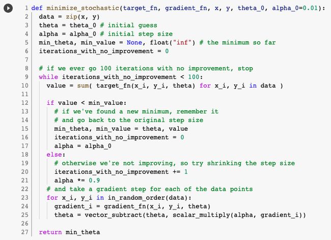
When this is the case, we can instead apply a technique called stochastic gradient descent, which computes the gradient (and takes a step) for only one point at a time. It cycles over our data repeatedly until it reaches a stopping point.
在这种情况下,我们可以改为应用一种称为随机梯度下降的技术,该技术一次只计算一个点的梯度(并采取一个步骤)。 它反复循环遍历我们的数据,直到达到停止点为止。
During each cycle, we’ll want to iterate through our data in a random order:
在每个周期中,我们要以随机顺序遍历数据:
And we’ll want to take a gradient step for each data point. This approach leaves the possibility that we might circle around near a minimum forever, so whenever we stop getting improvements we’ll decrease the step size and eventually quit:
我们将对每个数据点采取渐变步骤。 这种方法使我们有可能永远永远徘徊在最小值附近,因此,每当我们停止改进时,我们都会减小步长并最终退出:
The stochastic version will typically be a lot faster than the batch version. Of course, we’ll want a version that maximizes as well:
随机版本通常比批处理版本快很多。 当然,我们也需要一个最大化的版本:
I hope you found this article useful, Thank you for reading till here. If you have any question and/or suggestions, let me know in the comments.You can also get in touch with me directly through email & LinkedIn
希望本文对您有所帮助,谢谢您的阅读。 如果您有任何疑问和/或建议,请在评论中让我知道。您也可以通过电子邮件和LinkedIn直接与我联系
References and Further Reading
参考资料和进一步阅读
Hypothesis and Inference for Data Science
数据科学假设与推理
Linear Algebra for Data Science
数据科学的线性代数
Statistics for Data Science
数据科学统计
Probability for Data Science
数据科学的概率
翻译自: https://medium.com/swlh/gradient-descent-for-data-science-and-machine-learning-97528481513
机器学习之梯度与梯度下降法

