人工智能-强化学习-算法：PPO（Proximal Policy Optimization，改进版Policy Gradient）【PPO、PPO2、TRPO】

$$\begin{array}{r}\text{强化学习算法}\{\begin{array}{l}\text{Policy-Based Approach：Policy Gradient算法：Learning an Actor/Policy π}\\ \text{Value-based Approach：Critic}\{\begin{array}{l}\text{State value function Vπ(s)}\\ \\ \text{State-Action value function Qπ(s,a) ⟹ Q-Learning算法}\end{array}\\ \text{Actor+Critic}\end{array}\end{array}$$

OpenAI 把PPO当作他们默认强化学习算法

一、On-policy v.s. Off-policy

The on-policy approach in the preceding section is actually a compromise—it learns action values not for the optimal policy, but for a near-optimal policy that still explores. on-policy算法是在保证跟随最优策略的基础上同时保持着对其它动作的探索性，对于on-policy算法来说如要保持探索性则必然会牺牲一定的最优选择机会。

A more straightforward approach is to use two policies, one that is learned about and that becomes the optimal policy, and one that is more exploratory and is used to generate behavior. 有一个更加直接的办法就是在迭代过程中允许存在两个policy，一个用于生成学习过程的动作，具有很强的探索性，另外一个则是由值函数产生的最优策略，这个方法就被称作off-policy。

The policy being learned about is called the target policy, and the policy used to generate behavior is called the behavior policy.In this case we say that learning is from data “off” the target policy, and the overall process is termed off-policy learning.

1、On-policy Algorithm

• “要训练的Agent” 跟 “和环境互动的Agent” 是同一个的话，这个叫做 on-policy。即：要训练的Agent，它是一边跟环境互动，一边做学习这个叫 on-policy。比如：Policy Gradient。Policy Gradient 是一个会花很多时间来取样的算法。Policy Gradient 算法的大多数时间都在取样，Agent/Actor跟环境做互动取样后update参数一次(只能 update 参数一次)，接下来就要重新再去环境里取样，然后才能再次 update 参数一次，这非常花时间。

2、Off-policy Algorithm

• “要训练的Agent” 跟 “和环境互动的Agent” 不是同一个的话，这个叫做 off-policy。如果它是在旁边看别人玩，透过看别人玩，来学习的话，这个叫做 Off-policy。
• 在迭代过程中允许存在两个policy，${\pi }_{\theta }$，${\pi }_{{\theta }^{\prime }}$。其中 ${\pi }_{{\theta }^{\prime }}$ 一个用于生成学习过程的动作，具有很强的探索性，另外一个 ${\pi }_{\theta }$ 则是由值函数产生的最优策略，这个方法就被称作off-policy。
• 从 on-policy 变成 off-policy 的好处就是：用 ${\pi }_{{\theta }^{\prime }}$ 去跟环境做互动，用 ${\pi }_{{\theta }^{\prime }}$ 采样到的数据集去训练 ${\pi }_{\theta }$
• 用 ${\pi }_{{\theta }^{\prime }}$ 从环境中取样去训练 ${\pi }_{\theta }$ 意味着 ${\pi }_{{\theta }^{\prime }}$ 从环境中取的样可以用非常多次，${\pi }_{\theta }$ 在做梯度上升的时候，就可以执行梯度上升好几次，，${\pi }_{\theta }$ 可以 update 参数好几次，都只要用同一笔取样数据。，这样就会比较有效率

二、Importance Sampling

• off-policy与重要性采样(Importance Sampling)密不可分
• Importance Sampling主要的作用在于通过一个简单的可预测的分布去估计一个服从另一个分布的随机变量的均值。
• 在实际应用off-policy时，迭代过程通常会有两个策略，一个是Behavior policy，用于生成学习过程所需要选择的动作，这一个简单的，探索性非常强的关于动作选择的分布；另一个是Target policy，这是我们最终希望得到的最优动作选择分布。
• 应用Importance Sampling之处在于通过Behavior policy去估计Target policy可能反馈回来的收益的均值，即用一个简单分布去估计服从另一个分布的随机变量的均值。
• 如果可以从 $p(x)$ 分布取样时，
  $$\begin{array}{r}{E}_{x\sim p}[f(x)]\approx \frac{1}{N}\sum _{i=1}^{N}f(x_i)\end{array}$$
• 如果无法从 $p(x)$ 分布取样，但是可以从 $q(x)$ 分布取样时
  $$\begin{array}{r}{E}_{x\sim p}[f(x)]=\int f(x)p(x)dx=\int f(x)\frac{p(x)}{q(x)}q(x)dx=E_{x\sim q}[f(x)\frac{p(x)}{q(x)}]\end{array}$$
  其中的 $\frac{p(x)}{q(x)}$ 称为 Important Weight。
• 原则上，$p(x)$ 与 $q(x)$ 可以任意取，但是实践中，$p(x)$ 与 $q(x)$ 两分布要尽可能像，否则效果不好。因为 $f(x)$ 与 $f(x)\frac{p(x)}{q(x)}$ 的分布式不同的，如果取样无限次，则两者结果相同。但是在有限次取样后的结果是不同的。

三、On-policy算法(Policy Gradient) $\stackrel{ImportanceSampling}{}$ Off-policy算法

利用 Importance Sampling 将 Policy Gradient 这个 On-policy算法 转为 Off-policy算法

由Policy Gradient 可知：将 Policy Gradient 经过 “Add a Baseline”、“Assign Suitable Credit” 处理后的梯度为：

$$\begin{array}{rl}{\nabla }_{\theta }{\overline{R}}_{\theta }& \approx \frac{1}{N}\sum _{i=1}^N\sum _{t=1}^{T_i}[A^{\theta }(s_t,a_t){\nabla }_{\theta }log{p}_{\theta }(a_t^i|s_t^i)]\\ & =E_{(s_t,a_t)\sim {\pi }_{\theta }}[A^{\theta }(s_t,a_t){\nabla }_{\theta }log{P}_{\theta }(a_t|s_t)]\\ & =E_{(s_t,a_t)\sim {\pi }_{{\theta }^{\prime }}}\left[\frac{P_{\theta }(s_t,a_t)}{P_{{\theta }^{\prime }}(s_t,a_t)}{A}^{({\theta }^{\prime })}(s_t,a_t){\nabla }_{\theta }log{P}_{\theta }(a_t|s_t)\right]\\ & =E_{(s_t,a_t)\sim {\pi }_{{\theta }^{\prime }}}\left[\frac{P_{\theta }(a_t|s_t)P_{\theta }(s_t)}{P_{{\theta }^{\prime }}(a_t|s_t)P_{{\theta }^{\prime }}(s_t)}{A}^{({\theta }^{\prime })}(s_t,a_t){\nabla }_{\theta }log{P}_{\theta }(a_t|s_t)\right]\\ & \stackrel{令P_{\theta }(s_t)=P_{{\theta }^{\prime }}(s_t)}{}{E}_{(s_t,a_t)\sim {\pi }_{{\theta }^{\prime }}}\left[\frac{P_{\theta }(a_t|s_t)}{P_{{\theta }^{\prime }}(a_t|s_t)}{A}^{({\theta }^{\prime })}(s_t,a_t){\nabla }_{\theta }log{P}_{\theta }(a_t|s_t)\right]\\ & =E_{(s_t,a_t)\sim {\pi }_{{\theta }^{\prime }}}\left\{\left[\frac{P_{\theta }(a_t|s_t)}{P_{{\theta }^{\prime }}(a_t|s_t)}{A}^{({\theta }^{\prime })}(s_t,a_t)\right]{\nabla }_{\theta }log\left[\frac{P_{\theta }(a_t|s_t)}{P_{{\theta }^{\prime }}(a_t|s_t)}{A}^{({\theta }^{\prime })}(s_t,a_t)\right]\right\}\text{紫色部分与θ无关}\end{array}$$

$\text{∵}{\nabla }_{x}logf(x)=\frac{1}{f(x)}{\nabla }_{x}f(x)\text{∴}{\nabla }_{x}f(x)=f(x){\nabla }_{x}logf(x)$

$\text{∴}$目标函数为：
$$\begin{array}{r}{J}^{({\theta }^{\prime })}(\theta )={\overline{R}}^{({\theta }^{\prime })}(\theta )=E_{(s_t,a_t)\sim {\pi }_{{\theta }^{\prime }}}\left[\frac{P_{\theta }(a_t|s_t)}{P_{{\theta }^{\prime }}(a_t|s_t)}{A}^{({\theta }^{\prime })}(s_t,a_t)\right]\end{array}$$
其中：

• $\theta$ 表示待优化的参数；$\theta$不与环境互动；
• ${\theta }^{\prime }$ 表示用 ${\theta }^{\prime }$ 去做demonstration，${\theta }^{\prime }$ 与环境互动后取样 $(s_t,a_t)$，计算 $A^{({\theta }^{\prime })}(s_t,a_t)$

四、Off-policy算法 $\stackrel{AddConstraint}{}$ PPO/TRPO

• 由 “Importance Sampling” 的讨论可知，实践中，在公式 $\begin{array}{r}{E}_{x\sim p}[f(x)]=E_{x\sim q}[f(x)\frac{p(x)}{q(x)}]\end{array}$ 中的 $p(x)$ 与 $q(x)$ 两分布要尽可能像，否则效果不好。为了实现这个约束，需要在目标函数上加上一个约束条件。
• PPO 与 TRPO 的效果差不多，但是在实操时， 使用PPO算法 比 使用 TRPO 算法更容易操作。

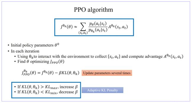
1、PPO (Proximal Policy Optimization)

$$\begin{array}{rl}{J}_{PPO}^{({\theta }^{\prime })}(\theta )& =J^{({\theta }^{\prime })}(\theta )-\beta KL(\theta ,{\theta }^{\prime })\\ & =E_{(s_t,a_t)\sim {\pi }_{{\theta }^{\prime }}}\left[\frac{P_{\theta }(a_t|s_t)}{P_{{\theta }^{\prime }}(a_t|s_t)}{A}^{({\theta }^{\prime })}(s_t,a_t)\right]-\beta KL(\theta ,{\theta }^{\prime })\end{array}$$
其中：

• $KL(\theta ,{\theta }^{\prime })$ 用来衡量 $\theta$ 与 ${\theta }^{\prime }$ 的相似度。
• $KL(\theta ,{\theta }^{\prime })$ 并不是表示 $\theta$与${\theta }^{\prime }$分布的距离，而是表示采用 $\theta$与${\theta }^{\prime }$这两个参数的两个Model的 Output 的 Action 的分布(即：${\pi }_{\theta }$与${\pi }_{{\theta }^{\prime }}$ 的分布) 的 KL-Divergence。
• 考虑的不是参数分布的KL-Divergence，而是利用各个参数产生的各个Action分布间的KL-Divergence，因为参数的变化与对应的Action的变化不一定完全一致。有时候你参数小小变了一下，它可能 output 的行为就差很多；或是参数变很多，但 output 的行为可能没什么改变。所以我们真正在意的是这个 actor 它的行为上的差距，而不是它们参数上的差距。
• 所以这里要注意一下，在做 PPO 的时候，所谓的 KL diversions 并不是参数的距离，而是 action 的距离。

2、TRPO (Trust Region Policy Optimization)

$$\begin{array}{r}{J}_{TRPO}^{({\theta }^{\prime })}(\theta )=E_{(s_t,a_t)\sim {\pi }_{{\theta }^{\prime }}}{\left[\frac{P_{\theta }(a_t|s_t)}{P_{{\theta }^{\prime }}(a_t|s_t)}{A}^{({\theta }^{\prime })}(s_t,a_t)\right]}_{KL({\pi }_{\theta },{\pi }_{{\theta }^{\prime }})<\delta }\end{array}$$

3、PPO2

$$\begin{array}{r}{J}_{PPO2}^{{\theta }_k}(\theta )\approx \sum _{(s_t,a_t)}min\left\{\frac{P_{\theta }(a_t|s_t)}{P_{{\theta }_k}(a_t|s_t)}{A}^{{\theta }_k}(s_t,a_t),clip\left[\frac{P_{\theta }(a_t|s_t)}{P_{{\theta }_k}(a_t|s_t)},1-\epsilon ,1+\epsilon \right]A^{{\theta }_k}(s_t,a_t)\right\}\end{array}$$

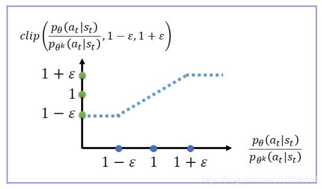
• PPO2算法的想法很直接，就是让 $P_{\theta }$ 与 $P_{{\theta }_k}$ 不要差距太大。也就是你拿来与环境互动做 demonstration 的那个 model，跟实际上 learn 的 model 最后在 optimize 以后，不要差距太大。
• 如果 $A^{({\theta }^{\prime })}(s_t,a_t)>0$，也就意味着该 $(s_t,a_t)$ 是好的，所以希望增加该 $(s_t,a_t)$ 的机率，所以想让 $p_{\theta }(s_t,a_t)$ 越大越好。但是 $\frac{p_{\theta }(s_t,a_t)}{p_{{\theta }_k}(s_t,a_t)}$ 比值不可以超过 $1+\epsilon$，如果超过 $1+\epsilon$ 的话，$p_{\theta }(s_t,a_t)$ 与 $p_{{\theta }_k}(s_t,a_t)$ 的差距就太大，就没有 benefit 了。所以今天在 train 的时候，$p_{\theta }(s_t,a_t)$只会被 train 到比 $p_{{\theta }_k}(s_t,a_t)$ 大 $1+\epsilon$ 倍就会停止
• 如果 $A^{({\theta }^{\prime })}(s_t,a_t)<0$，也就意味着该 $(s_t,a_t)$ 是坏的，所以希望减小该 $(s_t,a_t)$ 的机率，所以想让 $p_{\theta }(s_t,a_t)$ 越小越好。但是 $\frac{p_{\theta }(s_t,a_t)}{p_{{\theta }_k}(s_t,a_t)}$ 比值不可以小于 $1-\epsilon$，如果超过 $1-\epsilon$ 的话，$p_{\theta }(s_t,a_t)$ 与 $p_{{\theta }_k}(s_t,a_t)$ 的差距就太大，就没有 benefit 了。所以今天在 train 的时候，$p_{\theta }(s_t,a_t)$只会被 train 到比 $p_{{\theta }_k}(s_t,a_t)$ 小 $1-\epsilon$ 倍就会停止

4、PPO 跟其它方法的比較

在多数的 cases 里面，PPO 都是不错的，不是最好的，就是第二好的

---

---

---

参考资料：
深度增强学习PPO（Proximal Policy Optimization）算法源码走读
【RL系列】强化学习之On-Policy与Off-Policy
Sutton的Google硬盘
Proximal Policy Optimization Algorithms