用于Python降维的线性判别分析
减少预测模型的输入变量数称为降维。
较少的输入变量可以产生更简单的预测模型,该模型在对新数据进行预测时可能具有更好的性能。
线性判别分析(简称LDA)是一种用于多类分类的预测建模算法。它还可以用作降维技术,提供训练数据集的投影,以最好地按分配的类将示例分开。
使用线性判别分析进行降维的能力通常会让大多数从业者感到惊讶。
在本教程中,您将了解如何在开发预测模型时使用 LDA 进行降维。
完成本教程后,您将了解:
- 降维涉及减少建模数据中输入变量或列的数量。
- LDA 是一种多类分类技术,可用于自动执行降维。
- 如何评估使用 LDA 投影作为输入并使用新的原始数据进行预测的预测模型。
教程概述
本教程分为四个部分;它们是:
- 降维
- 线性判别分析
- LDA Scikit-Learn API
- LDA维数的工作示例
降维
降维是指减少数据集的输入变量数量。
如果数据是使用行和列表示的,例如在电子表格中,则输入变量是作为输入提供给模型以预测目标变量的列。输入变量也称为要素。
我们可以将表示 n 维特征空间上维度的数据列和数据行视为该空间中的点。这是对数据集的有用几何解释。
在具有 k 个数值属性的数据集中,您可以将数据可视化为 k 维空间中的点云......
— 第 305 页,数据挖掘:实用机器学习工具和技术,第 4 版,2016 年。
在特征空间中具有大量维度可能意味着该空间的体积非常大,反过来,我们在该空间中的点(数据行)通常代表一个小且不具代表性的样本。
这可能会极大地影响机器学习算法的性能,这些算法适合具有许多输入特征的数据,通常被称为“维度的诅咒”。
因此,通常需要减少输入要素的数量。这减少了特征空间的维数,因此称为“降维”。
降维的一种流行方法是使用线性代数领域的技术。这通常称为“特征投影”,使用的算法称为“投影方法”。
投影方法旨在减少特征空间中的维度数量,同时保留数据中观察到的变量之间最重要的结构或关系。
在处理高维数据时,通过将数据投影到捕获数据“本质”的低维子空间来降低维数通常是有用的。这称为降维。
— 第 11 页,机器学习:概率视角,2012 年。
然后,可以将生成的数据集(投影)用作训练机器学习模型的输入。
从本质上讲,原始特征不再存在,新特征是从与原始数据不直接可比的可用数据构建的,例如没有列名。
将来在进行预测时提供给模型的任何新数据(例如测试数据集和新数据集)也必须使用相同的技术进行投影。
线性判别分析
线性判别分析 (LDA) 是一种用于多类分类的线性机器学习算法。
它不应与“潜在狄利克雷分配”(LDA)混淆,后者也是文本文档的降维技术。
线性判别分析旨在通过类值最好地分离(或区分)训练数据集中的样本。具体而言,该模型寻求找到输入变量的线性组合,以实现类间样本的最大分离(类质心或均值)和每个类内样本的最小分离。
...查找预测变量的线性组合,以使组间方差相对于组内方差最大化。[...]查找预测变量的组合,这些预测变量在数据中心之间提供了最大的分离度,同时最小化了每组数据中的变异。
— 第 289 页,应用预测建模,2013 年。
有很多方法可以构建和解决LDA;例如,通常用贝叶斯定理和条件概率来描述LDA算法。
在实践中,用于多类分类的LDA通常使用线性代数中的工具实现,并且与PCA一样,使用矩阵分解作为技术的核心。因此,最好在拟合LDA模型之前对数据进行标准化。
有关如何详细计算 LDA 的详细信息,请参阅教程:
- 机器学习的线性判别分析
现在我们已经熟悉了降维和LDA,让我们看看如何将这种方法与scikit-learn库一起使用。
LDA Scikit-Learn API
我们可以使用 LDA 来计算数据集的投影,并选择投影的多个维度或组件作为模型的输入。
scikit-learn库提供了LinearDiscriminantAnalysis类,该类可以适应数据集,并用于将来转换训练数据集和任何其他数据集。
例如:
|
1
2
3
4
5
6
7
8
9
|
...
# prepare dataset
data = ...
# define transform
lda = LinearDiscriminantAnalysis()
# prepare transform on dataset
lda.fit(data)
# apply transform to dataset
transformed = lda.transform(data)
|
LDA 的输出可用作训练模型的输入。
也许最好的方法是使用管道,其中第一步是 LDA 转换,下一步是将转换后的数据作为输入的学习算法。
|
1
2
3
4
|
...
# define the pipeline
steps = [('lda', LinearDiscriminantAnalysis()), ('m', GaussianNB())]
model = Pipeline(steps=steps)
|
如果输入变量具有不同的单位或比例,则在执行 LDA 转换之前标准化数据也是一个好主意;例如:
|
1
2
3
4
|
...
# define the pipeline
steps = [('s', StandardScaler()), ('lda', LinearDiscriminantAnalysis()), ('m', GaussianNB())]
model = Pipeline(steps=steps)
|
现在我们已经熟悉了 LDA API,让我们看一个工作示例。
LDA维数的工作示例
首先,我们可以使用make_classification() 函数创建一个包含 1,000 个示例和 20 个输入特征的合成 10 类分类问题,其中 15 个输入是有意义的。
下面列出了完整的示例。
|
1
2
3
4
5
6
|
# test classification dataset
from sklearn.datasets import make_classification
# define dataset
X, y = make_classification(n_samples=1000, n_features=20, n_informative=15, n_redundant=5, random_state=7, n_classes=10)
# summarize the dataset
print(X.shape, y.shape)
|
运行该示例将创建数据集并汇总输入和输出组件的形状。
|
1
|
(1000, 20) (1000,)
|
接下来,我们可以在这个数据集上使用降维,同时拟合朴素贝叶斯模型。
我们将使用一个管道,其中第一步执行LDA变换并选择五个最重要的维度或组件,然后在这些特征上拟合朴素贝叶斯模型。我们不需要标准化此数据集上的变量,因为所有变量在设计上都具有相同的比例。
将使用重复分层交叉验证对管道进行评估,每次重复 3 次,每次重复 10 次。性能表示为平均分类准确度。
下面列出了完整的示例。
|
1
2
3
4
5
6
7
8
9
10
11
12
13
14
15
16
17
18
19
|
# evaluate lda with naive bayes algorithm for classification
from numpy import mean
from numpy import std
from sklearn.datasets import make_classification
from sklearn.model_selection import cross_val_score
from sklearn.model_selection import RepeatedStratifiedKFold
from sklearn.pipeline import Pipeline
from sklearn.discriminant_analysis import LinearDiscriminantAnalysis
from sklearn.naive_bayes import GaussianNB
# define dataset
X, y = make_classification(n_samples=1000, n_features=20, n_informative=15, n_redundant=5, random_state=7, n_classes=10)
# define the pipeline
steps = [('lda', LinearDiscriminantAnalysis(n_components=5)), ('m', GaussianNB())]
model = Pipeline(steps=steps)
# evaluate model
cv = RepeatedStratifiedKFold(n_splits=10, n_repeats=3, random_state=1)
n_scores = cross_val_score(model, X, y, scoring='accuracy', cv=cv, n_jobs=-1, error_score='raise')
# report performance
print('Accuracy: %.3f (%.3f)' % (mean(n_scores), std(n_scores)))
|
运行该示例将评估模型并报告分类准确性。
注意:根据算法或评估过程的随机性质或数值精度的差异,您的结果可能会有所不同。请考虑运行几次示例并比较平均结果。
在这种情况下,我们可以看到具有朴素贝叶斯的LDA变换实现了约31.4%的性能。
|
1
|
Accuracy: 0.314 (0.049)
|
我们怎么知道将 20 个输入维度减少到 5 个是好的还是我们能做的最好的?
我们没有;五是任意选择。
更好的方法是评估具有不同输入特征数的相同变换和模型,并选择可获得最佳平均性能的特征数(降维量)。
LDA 在降维中使用的分量数量限制在类数减去 1 之间,在这种情况下为 (10 – 1) 或 9
下面的示例执行此实验,并汇总了每个配置的平均分类准确性。
|
1
2
3
4
5
6
7
8
9
10
11
12
13
14
15
16
17
18
19
20
21
22
23
24
25
26
27
28
29
30
31
32
33
34
35
36
37
38
39
40
41
42
43
44
|
# compare lda number of components with naive bayes algorithm for classification
from numpy import mean
from numpy import std
from sklearn.datasets import make_classification
from sklearn.model_selection import cross_val_score
from sklearn.model_selection import RepeatedStratifiedKFold
from sklearn.pipeline import Pipeline
from sklearn.discriminant_analysis import LinearDiscriminantAnalysis
from sklearn.naive_bayes import GaussianNB
from matplotlib import pyplot
# get the dataset
def get_dataset():
X, y = make_classification(n_samples=1000, n_features=20, n_informative=15, n_redundant=5, random_state=7, n_classes=10)
return X, y
# get a list of models to evaluate
def get_models():
models = dict()
for i in range(1,10):
steps = [('lda', LinearDiscriminantAnalysis(n_components=i)), ('m', GaussianNB())]
models[str(i)] = Pipeline(steps=steps)
return models
# evaluate a give model using cross-validation
def evaluate_model(model, X, y):
cv = RepeatedStratifiedKFold(n_splits=10, n_repeats=3, random_state=1)
scores = cross_val_score(model, X, y, scoring='accuracy', cv=cv, n_jobs=-1, error_score='raise')
return scores
# define dataset
X, y = get_dataset()
# get the models to evaluate
models = get_models()
# evaluate the models and store results
results, names = list(), list()
for name, model in models.items():
scores = evaluate_model(model, X, y)
results.append(scores)
names.append(name)
print('>%s %.3f (%.3f)' % (name, mean(scores), std(scores)))
# plot model performance for comparison
pyplot.boxplot(results, labels=names, showmeans=True)
pyplot.show()
|
首先运行示例将报告所选每个组件或特征数的分类精度。
注意:根据算法或评估过程的随机性质或数值精度的差异,您的结果可能会有所不同。请考虑运行几次示例并比较平均结果。
随着维度数量的增加,我们可以看到性能提高的总体趋势。在此数据集上,结果表明在维度数与模型的分类准确性之间进行权衡。
结果表明,使用默认的九个组件可以在此数据集上实现最佳性能,尽管由于使用的维度较少,因此需要谨慎权衡。
|
1
2
3
4
5
6
7
8
9
|
>1 0.182 (0.032)
>2 0.235 (0.036)
>3 0.267 (0.038)
>4 0.303 (0.037)
>5 0.314 (0.049)
>6 0.314 (0.040)
>7 0.329 (0.042)
>8 0.343 (0.045)
>9 0.358 (0.056)
|
将创建箱须图,用于分布每个配置的维度数的精度分数。
我们可以看到分类准确性随着组件数量的增加而增加的趋势,限制为 9。
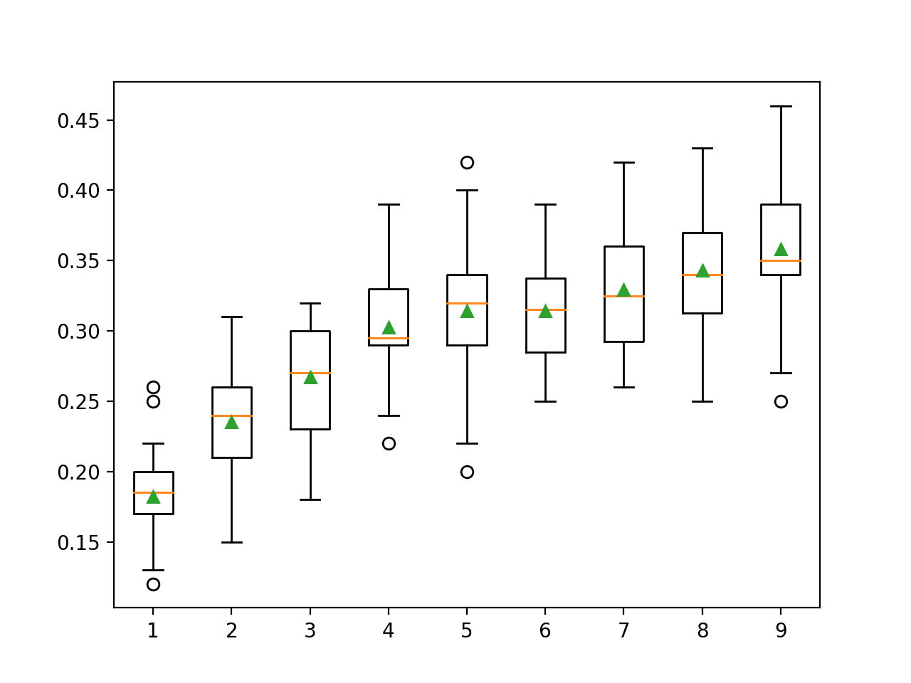
LDA 分量数与分类精度的箱形图
我们可以选择使用 LDA 变换和朴素贝叶斯模型组合作为我们的最终模型。
这涉及在所有可用数据上拟合管道,并使用管道对新数据进行预测。重要的是,必须对此新数据执行相同的转换,这些数据通过管道自动处理。
下面的代码提供了一个示例,说明如何拟合和使用最终模型,并对新数据进行 LDA 转换。
|
1
2
3
4
5
6
7
8
9
10
11
12
13
14
15
16
|
# make predictions using lda with naive bayes
from sklearn.datasets import make_classification
from sklearn.pipeline import Pipeline
from sklearn.discriminant_analysis import LinearDiscriminantAnalysis
from sklearn.naive_bayes import GaussianNB
# define dataset
X, y = make_classification(n_samples=1000, n_features=20, n_informative=15, n_redundant=5, random_state=7, n_classes=10)
# define the model
steps = [('lda', LinearDiscriminantAnalysis(n_components=9)), ('m', GaussianNB())]
model = Pipeline(steps=steps)
# fit the model on the whole dataset
model.fit(X, y)
# make a single prediction
row = [[2.3548775,-1.69674567,1.6193882,-1.19668862,-2.85422348,-2.00998376,16.56128782,2.57257575,9.93779782,0.43415008,6.08274911,2.12689336,1.70100279,3.32160983,13.02048541,-3.05034488,2.06346747,-3.33390362,2.45147541,-1.23455205]]
yhat = model.predict(row)
print('Predicted Class: %d' % yhat[0])
|
运行该示例会针对所有可用数据拟合管道,并对新数据进行预测。
在这里,转换使用了 LDA 转换中九个最重要的组件,正如我们从上面的测试中发现的那样。
提供一行包含 20 列的新数据,并自动转换为 15 个分量并馈送到朴素贝叶斯模型,以预测类标签。
|
1
|
Predicted Class: 6
|