吴恩达机器学习课后 lab C1_W1_Lab03_Cost_function_Soln-checkpoint
C1_W1_Lab03_Cost_function_Soln-checkpoint (代价函数)
- 代码块1
- 代码块2
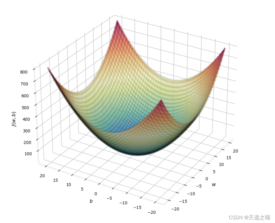
- 代价函数
- 代码块3
- 代码块4(可视化代价函数)
- 代码块5
- 代码块6
- 代码块7
- 总结
代码块1
import numpy as np
%matplotlib widget#这个模块是matplotlib中的GUI模块,可以通过调整bottom来实时改变显示的结果
import matplotlib.pyplot as plt
from lab_utils_uni import plt_intuition,
#导入一些包
plt_stationary, plt_update_onclick, soup_bowl
plt.style.use('./deeplearning.mplstyle')
代码块2
x_train = np.array([1.0, 2.0])           #(size in 1000 square feet)
y_train = np.array([300.0, 500.0])           #(price in 1000s of dollars)
定义了两个一维数组
代价函数
代码块3
def compute_cost(x, y, w, b):
    """
    Computes the cost function for linear regression.
    Args:
      x (ndarray (m,)): Data, m examples
      y (ndarray (m,)): target values
      w,b (scalar)    : model parameters
    Returns
        total_cost (float): The cost of using w,b as the parameters for linear regression
               to fit the data points in x and y
    """
    # number of training examples
    m = x.shape[0]

    cost_sum = 0
    for i in range(m):
        f_wb = w * x[i] + b
        cost = (f_wb - y[i]) ** 2
        cost_sum = cost_sum + cost
    total_cost = (1 / (2 * m)) * cost_sum

    return total_cost
计算代价函数
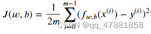
代码块4(可视化代价函数)
plt_intuition(x_train,y_train)
输出
调整w可以达到拟合样本的效果
代码块5
x_train = np.array([1.0, 1.7, 2.0, 2.5, 3.0, 3.2])
y_train = np.array([250, 300, 480,  430,   630, 730,])
更大的数据集
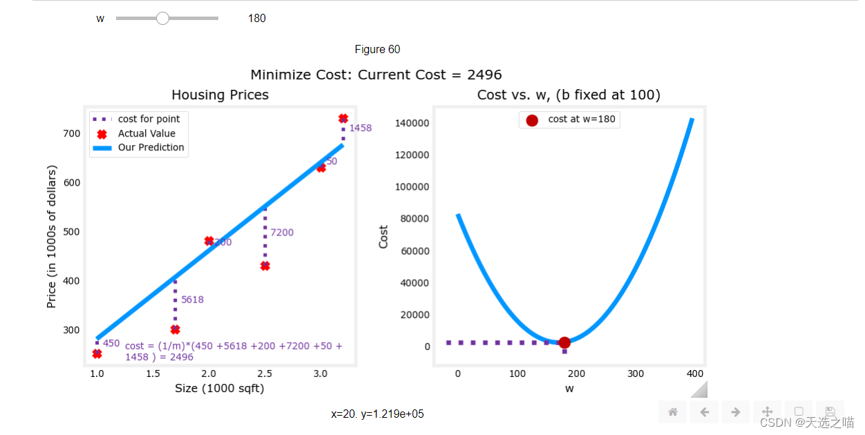
代码块6
plt.close('all') #关闭上面绘图
fig, ax, dyn_items = plt_stationary(x_train, y_train)
updater = plt_update_onclick(fig, ax, x_train, y_train, dyn_items)
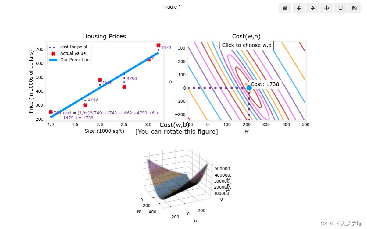
代码块7
成本函数平方损失的事实确保了“误差面”像汤碗一样凸起。它总是有一个最小值,可以通过在所有维度上遵循梯度来达到。在前面的图中,因为 和 维度的比例不同,这不容易识别。下图,其中 和 是对称的
soup_bowl()
总结
最小化代价函数