vae 实现
Since its introduction in 2013 through this paper, variational auto-encoder (VAE) as a type of generative model has stormed the world of Bayesian deep learning with its application in a wide range of domains. The original paper by Kingma and Welling has over 10k citations; meanwhile, as its construction might not appear to be straightforward to digest at the first glance, there have been numerous great articles explaining the intuition, architecture, and other different components of the model.
自从2013年通过本文引入变分自动编码器(VAE)作为一种生成模型以来,它在广泛领域中的应用席卷了贝叶斯深度学习领域。 Kingma和Welling的原始论文被引用了1 万多个 ; 同时,由于乍一看它的构造可能似乎不容易理解,因此有许多很棒的文章解释了模型的直觉,体系结构和其他不同组成部分。
However, the implementation of VAE usually comes as a complement to those articles, and the code itself is less talked about, especially being contextualized under some specific deep learning library (TensorFlow, PyTorch, etc.) — meaning that the code is just put out there in a code block, without enough comments about how some arguments work, why choose this particular function over others, etc. Also, due to the flexibility of each of these popular libraries, you might find these demo VAE implementations all appear different from each other. Furthermore, some versions might be implemented incorrectly, even by one of TensorFlow’s own tutorials (I will address this post later, mainly under Version a. of my implementation), but the mistakes might not be caught without comparison to other versions. Lastly, it’s of course nice to follow through one version that works, but I barely came across a post that compares laterally different ways of implementation. All of these motivate me to write this post.
但是,VAE的实现通常是对这些文章的补充,并且代码本身很少被谈论,尤其是在某些特定的深度学习库(TensorFlow,PyTorch等)下进行上下文化-这意味着代码刚刚发布在代码块中,没有足够的注释来说明某些参数的工作方式,为什么选择此特定函数而不是其他函数,等等。此外,由于每个流行的库的灵活性,您可能会发现这些演示版VAE实现看上去每个都不同其他。 此外,即使使用TensorFlow自己的教程之一 ,某些版本的实现也可能不正确(我将在稍后的内容中介绍该帖子,主要是在实现的a。版中 ),但是如果不与其他版本进行比较,就不会发现错误。 最后,遵循一个可行的版本当然很高兴,但是我几乎没有遇到过比较横向不同的实现方式的文章。 所有这些促使我写这篇文章。
This post is by no means an intro to VAE — I’d assume the reader has already had some level of understanding of how VAE works, and wants to know more about the implementation side of things.
这篇文章绝不是VAE的简介-我认为读者已经对VAE的工作方式有了一定的了解,并且想了解更多有关实现方面的知识。
I plan to divide this post into two components, which together completes the title:
我打算将这篇文章分为两个部分,共同完成标题:
Things to pay extra attention to when implementing VAE in general, using TF2 and TFP
通常 ,使用TF 2和TFP 实施VAE时要特别注意
How to implement VAE in different ways, using TF2 and TFP
如何使用TF 2和TFP 以不同方式实施VAE
Before I start to dive into each part, I want to use the following two paragraphs to share my personal experience of studying this model:
在开始研究每个部分之前,我想使用以下两段来分享我学习该模型的个人经验:
I’d thought that I had a good understanding of the model after reading the paper, until I started to implement it. When reading the paper, there are usually so many details about the model that one might very likely lose track on the parts to pay extra attention upon. Sometimes, a component of the model that the paper spent one short sentence on might take me hours to fully grasp and to make it work during implementation. In my opinion, if you want to have a good understanding on how a model works, although it’s definitely nice to try to go through the paper as thoroughly as possible, it’s IMHO better to try to implement it yourself.
在开始阅读本文之前,我以为我对模型有了很好的了解,直到开始实施它为止。 阅读本文时,通常会有太多关于模型的细节,以至于人们很可能会失去对零件的关注,从而需要格外注意。 有时,本文花了一句话简短描述的模型的一部分可能要花我几个小时才能完全掌握并使其在实施过程中起作用。 我认为,如果您想对模型的工作原理有一个很好的了解,尽管尝试尽可能彻底地研究本文绝对是一件好事,但IMHO最好自己尝试实现。
When you start to implement the model, I’d say pick a benchmark dataset that the community already know how the model would behave towards, instead of trying to come up with your own dataset, especially if you are implementing the model for the first time. This is particularly important, as you’d have a very clear goal about how the results would look like — a reference so to speak. Because simply making the code run without error, and seeing the cost drop is far from calling the implementation a working one yet; we need to at least see if it behaves in a certain way that others have already observed on a particular dataset.
当您开始实施模型时,我想说的是选择一个社区已经知道该模型将如何表现的基准数据集,而不是尝试提出自己的数据集,特别是如果您是第一次实施模型时。 这一点特别重要,因为您将对结果的外观有一个非常明确的目标-可以这么说。 因为简单地使代码运行没有错误,并且看到成本下降还远远不能将实现称为可行的实现。 我们至少需要查看它是否以其他人已经在特定数据集上观察到的特定方式运行。
第0部分:阐明实施目标 (Part 0: Clarifying the Implementation Goal)
Per the discussion from the above section, I will introduce the dataset, as well as the particular tasks for the VAE model to accomplish. For this post, I applied MNIST dataset with handwritten digits, with images of shape (28,28,1). I preprocessed it by normalizing the dataset to be between 0 and 1, and discretized the values to be either 0 or 1, using 0.5 as threshold. The tasks for the VAE model to accomplish on this dataset are:
根据上一节的讨论,我将介绍数据集,以及VAE模型要完成的特定任务。 对于这篇文章,我将MNIST数据集应用于手写数字,图像形状为(28,28,1) 。 我通过将数据集标准化为0到1对其进行了预处理,并使用0.5作为阈值将值离散化为0或1 。 VAE模型要在此数据集上完成的任务是:
(a) Reconstruction of the input digit images as close as possible
(a) 尽可能近地重建输入数字图像
(b) Generation of new digit images that look realistic, using random samples from the prior distribution (rather than samples from the posterior, conditional on data) as the input to the decoder
(b)使用来自先验分布的随机样本(而不是来自后验的样本,以数据为条件)作为解码器的输入,生成看起来逼真的新数字图像
Task (a) is relatively easy to accomplish, however Task (b) is, in my opinion, the one that indicates if the implementation works: that it has learnt the multimodality of different digits from the training data, and is able to produce new digit images as a generative model.
任务(a)相对容易完成,但是我认为任务(b)是一种指示实施是否可行的任务:它已从训练数据中学到了不同数字的多模态,并能够产生新的数字图像作为生成模型。
Now we are ready to dive into each component of this post.
现在,我们准备深入探讨本文的每个组成部分。
第一部分:实施VAE时的主要重点 (Part I: Main Focus when Implementing VAE)
Two things, both w.r.t. the loss function for each instance:
两件事,每个实例都有损失函数:
The loss function consists of two parts: the reverse KL divergence (between prior and posterior distribution of the latent variable z), and the expected negative log-likelihood (of the decoder distribution on the data to be reconstructed; also called the expected reconstruction error). Adding these two parts together, we get negative ELBO, which is to be minimized. For the computation of each part, we need to pay extra attention to what operation (taking the sum vs. taking the mean) we need to do on each dimension of data.
损失函数由两部分组成:反向KL散度(潜变量z的先验分布和后验分布)和预期的负对数似然(解码器对要重建的数据的分布);也称为预期重建误差)。 将这两个部分加在一起,我们得到负ELBO,这将被最小化。 对于每个部分的计算,我们需要特别注意在数据的每个维度上需要执行的操作(取总和取平均值)。
The weight of KL divergence in the loss function is a hyperparameter we shouldn’t ignore at all: it adjusts the “distance” between prior and posterior distribution of z, and plays a decisive role in the performance of the model.
损失函数中KL散度的权重是一个我们绝对不应该忽略的超参数:它调整z的前后分布之间的“距离”,并在模型的性能中起决定性作用。
Here is the loss function:
这是损失函数:
The computation of this loss function can be done in various ways, and is often very prone to make mistakes during implementation, especially w.r.t. what’s mentioned in the first bullet point: the operations on each dimension of data. I will elaborate on it in Part II, where each way of the implementation is introduced separately.
损失函数的计算可以通过多种方式完成,并且在实现过程中经常很容易出错,尤其是在第一个要点提到的内容:对数据各个维度的操作。 我将在第二部分中对此进行详细说明,其中分别介绍每种实现方式。
Notice that it shall actually be the loss function for Beta-VAE, in which ω can take values other than 1. This hyperparameter is crucial, especially when for Task (b) mentioned in Part 0: what this hyperparameter does is that it decides how hard we want to penalize the difference between the prior and posterior distribution of z. A lot of times the reconstruction of images would look perfect, while the generation from code z sampled from its prior would have all kinds of crazy looks. If ω is set to be too small, we are basically not regularizing the posterior at all, thus after training it might be drastically different from the prior — in the sense that z sampled from the prior would often fall into the area with very low density in the posterior distribution. As a result, the decoder would not know what to do with such samples of z, as it’s trained on z from the posterior distribution (note the distribution at the subscript of the expectation for the negative log-likelihood term from the loss function above). Here are the reconstructed and generated digits when ω=0.0001:
注意,它实际上应该是Beta-VAE的损失函数,其中ω可以取非1的值。 此超参数至关重要,尤其是对于第0部分中提到的任务(b)而言 :此超参数的作用是决定我们要如何难于补偿z的先验分布与后验分布之间的差异。 很多时候,图像的重建看起来是完美的,而从其先前采样的代码z生成的图像将具有各种疯狂的外观。 如果将ω设置得太小,我们基本上根本就不会对后验进行正则化,因此在训练后,它可能与前验有很大不同-在某种意义上,从前验采样的z通常会落入密度非常低的区域在后部分布。 结果,解码器将不知道如何处理z的这些样本,因为它是从后验分布对z进行训练的(请注意,根据上述损失函数得出的对数似然项的期望的下标分布) 。 这是ω= 0.0001时重构和生成的数字:
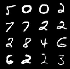
Notice that reconstructed digits can be clearly distinguished (and also match their labels), but the generated digits are basically dark and unrecognizable. This is an example of under-regularization.
请注意,可以清楚地区分重构的数字(并与它们的标签相匹配),但是生成的数字基本上是黑暗且无法识别的。 这是监管不足的一个例子。
On the other hand, if ω is too large, the posterior would be pulled too close to the prior, thus no matter what image is inputed to the encoder, we’d end up getting a z as if it’s randomly sampled from the prior. Here are the reconstructed and generated digits when ω=20:
另一方面,如果ω太大,则后验将被拉得离先验太近,因此,无论将什么图像输入到编码器,我们最终都会得到一个z,就像从先验中随机取样一样。 这是ω= 20时重构和生成的数字:
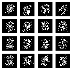
Notice that all digits look the same, no matter if it’s reconstructed conditional on the input digit, or generated as a new digit. This is an example of over-regularization.
请注意,无论数字是根据输入数字重建还是作为新数字生成,所有数字看起来都相同。 这是过度规范化的一个例子。
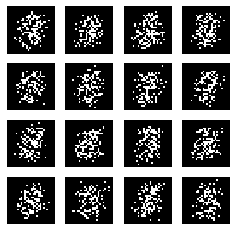
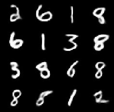
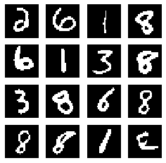
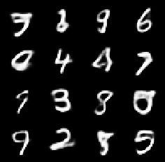
Thirdly, we have the scenario when ω is set to be “just the right amount” — in the sense that the posterior is distinct enough from the prior to be flexible conditioning on the input digit data, thus the reconstruction looks great; while the high-density areas of the two distributions have enough overlap, hence the z samples from the prior wouldn’t look too unfamiliar to the decoder as its input. Here are the reconstructed and generated digits when ω=3:
第三,假设ω被设置为“恰好合适的数量”,即后验与先验有足够的区别,从而可以灵活地对输入数字数据进行条件调整,因此重构看起来很棒; 虽然两个分布的高密度区域具有足够的重叠,所以来自先验的z个样本对于解码器作为其输入看起来不会太陌生。 这是ω= 3时重构和生成的数字:
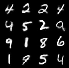
Notice that all reconstructed and most of generated digits appear to be recognizable, while some of the generated digits appear less realistic.
请注意,所有重构的数字和大多数生成的数字似乎都是可识别的,而某些生成的数字看起来不太现实。
In summary, while the autoencoder setup places a information bottleneck upon the latent variable z, forcing it to keep only the most essential information needed to reconstruct x after dimension reduction, ω helps to place z at the space that can make the decoder generate new x from scratch that would look like real x, while maintaining the quality of reconstruction.
总而言之,虽然自动编码器设置将信息瓶颈置于潜在变量z上 ,迫使其仅保留降维后重建x所需的最基本信息,但ω有助于将z置于可以使解码器生成新x的空间从头开始看起来像真实的x,同时保持重建的质量。
有点离题:TensorFlow 2和TensorFlow概率 (A little digression: TensorFlow 2 and TensorFlow Probability)
You might notice that although I put these two libraries in my title, the post so far has focused purely on discussing the VAE model and its application on MNIST dataset. I originally wanted to write about TF2 and TFP as the third component when I structured the post, but then I decided to contextualize them, i.e. to talk about them while I go through the implementation details in Part I and Part II. However, it could appear too hasty if I jump right into the code without giving a little background on these libraries. So here they come.
您可能会注意到,尽管我将这两个库放在标题中,但到目前为止,该帖子仅专注于讨论VAE模型及其在MNIST数据集上的应用。 构建帖子时,我本来希望将TF 2和TFP作为第三部分来撰写,但是后来我决定将它们进行上下文化,即在我阅读第一部分和第二部分中的实现细节时谈论它们。 但是,如果我直接进入代码而又不对这些库有一点背景知识的话,可能显得太草率了。 所以他们来了。
TF2
TF2
TensorFlow 2.0.0 was released in late September, 2019 — so it’s not even a year since its initial release. The latest version at the moment is 2.3.0, released in July, 2020. I started to work on a research project that had me pick up TF2 in November last year, thus I’ve used all four versions so far, each for a little while. At the time I was fully aware that PyTorch had been gaining a lot of traction in the research community; I chose TF2 mainly because it was the library where the project’s codebase was built upon.
TensorFlow 2.0.0于2019年 9月下旬发布-距其首次发布还不到一年。 目前的最新版本是2.3.0 ,于2020年 7月发布。 去年11月,我开始从事一个研究项目,让我拿起TF 2 ,因此到目前为止,我已经使用了所有四个版本,每个版本都有一段时间。 那时,我充分意识到PyTorch在研究界已经获得了很大的吸引力。 我之所以选择TF 2,主要是因为它是构建项目代码库的库。
My first impression of TF2: it was indeed much more convenient to develop deep learning models than TF1. With eager execution being one of its most distinctive features that separate TF2 from TF1, I no longer need to build the entire computational graph without seeing any intermediate results, which makes debugging a disaster as there’s no easy way to decompose each step and test its output. While the eager execution might come with the compromise to model training speed, the decorator @tf.function helps to some extent restore the efficiency under graph mode. Furthermore, its integration with Keras has brought some great perks — the Sequential and Functional API have brought different levels of flexibility when stacking up the neural network (NN) layers, just like their equivalents under PyTorch, torch.nn.Sequential and torch.nn.functional; also as a high level API, its interface looks deceptively simple (to the point that it’d cause trouble during VAE implementation — check my discussion under the implementation Version a. in Part II), as if I’m training a scikit-learn model.
我对TF 2的第一印象:开发深度学习模型确实比TF 1方便得多。 急切的执行是将TF 2与TF 1分开的最鲜明的功能之一,我不再需要构建完整的计算图而不会看到任何中间结果,这使调试成为一种灾难,因为没有简单的方法可以分解每个步骤并进行测试它的输出。 尽管急于执行可能会降低模型训练速度,但装饰器@tf.function在某种程度上有助于恢复图形模式下的效率。 此外,它与Keras的集成带来了很多好处-顺序和功能API在堆叠神经网络(NN)层时带来了不同级别的灵活性,就像在PyTorch, torch.nn.Sequential和torch.nn.functional下的等效物torch.nn.functional ; 作为高级API,它的界面看起来也很简单(以至于在VAE实施过程中会造成麻烦-请查看第二部分中的 版本a。下的讨论),就好像我正在训练scikit-learn模型。
Meanwhile, since it has only been less than a year since its first release, it’s definitely not as stable as I’d hope from a popular library. I still remembered that I got stuck over some simple tensor indexing procedure: I implemented the same functionality in multiple versions, which all led me to the same error message; however, it was such a straightforward step that no one would expect it to be the place that causes error. It turned out that after updating TF version to 2.1.0 after its release in early January this year, the model worked without changing any code. The most recent example was when adding a Dense layer after flattening the tensor, I got an error message regarding dimension, which also went away when updating TF version from 2.2.0 to 2.3.0.
同时,由于自首次发布以来不到一年,所以它绝对不如我所希望的那样受欢迎。 我仍然记得我被一些简单的张量索引过程困住了:我在多个版本中实现了相同的功能,这都导致了相同的错误消息; 但是,这是一个非常简单的步骤,没有人会期望它是导致错误的地方。 事实证明,在今年1月初发布TF版本并将其更新为2.1.0之后,该模型无需更改任何代码即可工作。 最近的示例是在拉平张量后添加Dense层时,出现有关尺寸的错误消息,当将TF版本从2.2.0更新到2.3.0时,该错误消息也消失了。
Furthermore, its user and developer community have not been as active as I expected. I’ve posted multiple questions under Keras Github Issues page, including the one mentioned above — all ended up with me answering my own question and closing the issue. Some issues obtained comments from users after several months, but none was addressed by the TensorFlow/Keras team.
此外,它的用户和开发人员社区没有我期望的那么活跃。 我在“ Keras Github问题”页面下发布了多个问题,包括上面提到的一个 问题 ,所有问题最终都由我回答自己的问题并结束。 几个月后,一些问题获得了用户的评论,但TensorFlow / Keras团队未解决任何问题。
Lastly, some of its documentation has not been straightforward or organized enough to follow. I’ve spent a lot of time trying to figure out how the decorator @tf.function actually works, and eventually I concluded that the best way is just trying to imitate the working examples without caring too much about the rationale at the moment. Some of its tutorials have also appear to be sloppy or even misleading (by giving incorrect implementation) — I will give examples later.
最后,它的某些文档还不够简单明了或组织不足以遵循。 我花了很多时间试图弄清楚装饰器@tf.function实际工作方式,最后我得出结论,最好的方法是尝试模仿工作示例,而无需过多关注当前的原理。 它的某些教程似乎也很草率,甚至具有误导性(通过提供不正确的实现方式),我将在后面给出示例。
TFP
全要素生产率
TensorFlow Probability was introduced in the first half of 2018, as a library developed specifically for probabilistic modeling. It implements the reparameterization trick under the hood, which enables backpropagation for training probabilistic models. You can find a good demonstration of the reparameterization trick in both the VAE paper and this paper that proposed Bayes by Backprop algorithm — the former work has the hidden nodes for the latent variable z and the output nodes of the decoder being probabilistic, while the latter one has the learnable parameters (weights and biases of each NN layer) being probabilistic.
TensorFlow概率于2018年上半年引入,是专门为概率建模开发的库。 它在引擎盖下实施了重新参数化技巧,从而可以进行反向传播以训练概率模型。 您可以在VAE论文和通过Backprop算法提出贝叶斯的 论文中找到关于重新参数化技巧的很好的演示-前一项工作具有潜在变量z的隐藏节点,而解码器的输出节点具有概率,而后者一个具有可学习参数(每个NN层的权重和偏差)的概率。
With TFP, we no longer need to explicitly define the mean and variance parameter for the posterior distribution of z, nor the computation of KL divergence, which greatly simplifies the code. As a matter of fact, it might make the implementation too simple that one could do it without having a great understanding of VAE, because its major components that would require a good grasp to the model are basically all abstracted by TFP. As a result, mistakes can also be easily made when using TFP to implement VAE as well.
使用TFP,我们不再需要为z的后验分布显式定义均值和方差参数,也无需计算KL散度,从而大大简化了代码。 实际上,它可能会使实现变得过于简单,以至于在不完全了解VAE的情况下就可以做到这一点,因为需要很好地掌握模型的主要组件基本上都是TFP所抽象的。 结果,在使用TFP实施VAE时,也很容易出错。
I’d suggest that you start by explicitly implementing the reparameterization trick and defining the KL term, if it’s your first time implementing VAE and that you want to know well about how the model works — I will start with this way of implementation as the first version in Part II.
我建议您从明确实现重新参数化技巧并定义KL术语开始,如果这是您第一次实现VAE,并且您想充分了解模型的工作原理,那么我将首先从这种实现方式开始第二部分的版本。
第二部分:实施VAE的不同方法 (Part II: Different Ways of Implementing VAE)
Before diving into the details of each implementation version, I’d like to list all of them here first. This list is by no means exhaustive, but rather representative to the points I plan to make.
在深入探讨每个实现版本的细节之前,我想先在这里列出所有它们。 该列表绝不是详尽无遗的,而是代表了我计划提出的观点。
The various way of implementing VAE are due to the different options we have for each of the following 3 modules:
实施VAE的方式多种多样,是因为我们为以下3个模块中的每个模块提供了不同的选择:
- the output layer of encoder 编码器的输出层
- the output layer of decoder 解码器的输出层
- the loss function (mainly the part that computes the expected reconstruction error) 损失函数(主要是计算预期重构误差的部分)
Each module has options as follows:
每个模块具有以下选项:
编码器的输出层 (the output layer of encoder)
tfpl.IndependentNormaltfpl.IndependentNormaltfkl.Densethat outputs (concatenated) mean and (raw) standard deviation of the posterior distribution of ztfkl.Dense,输出z的后验分布的(串联)均值和(原始)标准偏差
解码器的输出层 (the output layer of decoder)
tfpl.IndependentBernoullitfpl.IndependentBernoullitfpl.IndependentBernoulli.meantfpl.IndependentBernoulli.meantfkl.Conv2DTransposethat outputs the logitstfkl.Conv2DTranspose输出日志
损失函数 (the loss function)
negative_log_likelihood = lambda x, rv_x: -rv_x.log_prob(x)negative_log_likelihood = lambda x, rv_x: -rv_x.log_prob(x)tf.nn.sigmoid_cross_entropy_with_logitstf.nn.sigmoid_cross_entropy_with_logitstfk.losses.BinaryCrossentropytfk.losses.BinaryCrossentropytf.nn.sigmoid_cross_entropy_with_logits+tfkl.Layer.add_losstf.nn.sigmoid_cross_entropy_with_logits+tfkl.Layer.add_lossPyTorch-esque explicit computation by epoch through
with tf.GradientTape() as tape+tf.nn.sigmoid_cross_entropy_with_logits+tfkl.Layer.add_loss通过纪元通过
with tf.GradientTape() as tape+tf.nn.sigmoid_cross_entropy_with_logits+tfkl.Layer.add_loss来with tf.GradientTape() as tape式的显式计算PyTorch-esque explicit computation by epoch through
with tf.GradientTape() as tape+tf.nn.sigmoid_cross_entropy_with_logits通过纪元通过
with tf.GradientTape() as tape+tf.nn.sigmoid_cross_entropy_with_logits来with tf.GradientTape() as tape式的显式计算
Side note:
边注:
we have the following module abbreviations:
我们有以下模块缩写:
import tensorflow as tfimport tensorflow_probability as tfptfd = tfp.distributionstfpl = tfp.layerstfk = tf.kerastfkl = tf.keras.layers
导入tensorflow为tf导入tensorflow_probability为tfptfd = tfp.distributionstfpl = tfp.layerstfk = tf.kerastfkl = tf.keras.layers
Also note that the NN architecture of the encoder and the decoder are of less importance — I use the same architecture as this TF tutorial for all versions of my implementation.
还要注意,编码器和解码器的NN体系结构不太重要-在我的实现的所有版本中,我都使用与此TF教程相同的体系结构。
One might think that since the computation of KL divergence can be done differently (analytical solution vs. MC approximation), it should also be a module; but since the way to implement this term is more or less determined by the choice of the decoder output layer, and adding it as the fourth module might over-complicate the presentation, I choose to talk about it under one of the implementation versions (Version a.) instead.
可能有人认为,由于KL散度的计算可以不同地进行(解析解与MC近似),因此它也应该是一个模块。 但是由于实现此术语的方式或多或少取决于解码器输出层的选择,并且将其添加为第四个模块可能会使演示过于复杂,因此我选择在一种实现版本( 版本a。 )代替。
The implementations are simply the combinatorics of different options from each of the 3 modules:
这些实现只是3个模块中每个模块的不同选项的组合:
Now let’s dive into each version of implementation.
现在,让我们深入研究实现的每个版本。
版本a。 (Version a.)
This version is perhaps the most widely adopted one — as far as I know, all of my fellow researchers have been writing in this way: the encoder outputs nodes that represent the mean and (some transformation of, with range in ℝ) the standard deviation of the posterior distribution of the latent variable z. We then use the reparameterization trick to sample z as follows (from Equation (10) of VAE paper):
此版本可能是使用最广泛的版本-据我所知,我所有的研究人员都是以这种方式编写的:编码器输出的节点代表均值和(以some为单位的某种变换)标准偏差变量z的后验分布 然后,我们使用重新参数化技巧对z进行如下采样(来自VAE纸的公式(10) ):

in which ϵ is sampled from a standard multivariate Gaussian distribution, and the mean and the standard deviation of the posterior distribution q are outputted deterministically from the encoder. The obtained z is then used as the input to the decoder. Since after preprocessing our image data x is binary, it’s natural to assume a multivariate Bernoulli distribution (where all pixels are independent with each other) whose parameters are the output of the decoder — this is the scenario described under Appendix C.1 Bernoulli MLP as decoder in the VAE paper. Therefore, the log-likelihood of the decoder distribution has the following form (Equation (11) of the VAE paper):
其中ϵ是从标准多元高斯分布中采样的,后验分布q的均值和标准偏差是从编码器确定性输出的。 然后将获得的z用作解码器的输入。 由于在对图像数据x进行预处理之后,我们很自然地假设了一个多元伯努利分布(所有像素彼此独立),其参数是解码器的输出-这是附录C.1伯努利MLP中描述的情况: VAE文件中的解码器 。 因此,解码器分布的对数似然具有以下形式(VAE论文的等式(11) ):
in which y is the decoder output as the Bernoulli parameters for each pixel, and D is the number of pixels for each instance. z here represents a single sample from the encoder; since the expected negative log-likelihood term in the loss function cannot be computed analytically, we use MC approximation as follows (from Equation (10) of the VAE paper):
其中y是解码器输出,作为每个像素的伯努利参数, D是每个实例的像素数。 z代表编码器的单个样本; 由于无法通过解析计算损失函数中预期的负对数似然项,因此我们按如下方式使用MC近似(来自VAE论文的公式(10) ):
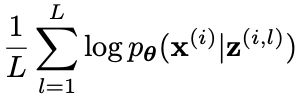
in which the z term (with the exact same form of superscript as the one in the reparameterization trick equation above) represents the l-th MC sample for the i-th digit image instance. In practice, it’s usually enough to set L=1, i.e. only one MC sample is needed.
其中z项(与上面的重新参数化技巧方程式的形式完全相同的上标形式)表示第i个数字图像实例的第l个MC样本。 实际上,设置L = 1通常就足够了,即仅需要一个MC样本。
The other term in the loss function, the reverse KL divergence, can also be approximated through MC samples. Since we assume the encoder distribution q to be multivariate Gaussian, we can directly plug the mean and variance outputted by the encoder into its density function:
损失函数中的另一项,即反向KL散度,也可以通过MC样本来近似。 由于我们假设编码器分布q为多元高斯,因此我们可以将编码器输出的均值和方差直接插入其密度函数中:
in which f represents the multivariate Gaussian density. Similarly, we can set L=1 as well in practice.
其中f代表多元高斯密度。 同样,在实践中我们也可以设置L = 1 。
Furthermore, if we let q to be multivariate Gaussian with a diagonal covariance matrix, the KL divergence term can be computed analytically as shown in Appendix B of the VAE paper:
此外,如果让q为具有对角协方差矩阵的多元高斯,则可以按照VAE论文附录B所示分析计算KL散度项:
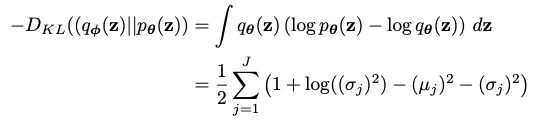
in which J represents the number of dimensions of z.
其中J表示z的维数。
In this version of implementation, I put the code that computes the cost of a mini-batch image data (note that the loss function is computed on a single instance; the cost function is the average of losses for all instances) into the function vae_cost, and define the optimization step at each epoch through function train_step. Here’s how they are implemented in TF2:
在此版本的实现中,我将计算小批量图像数据成本的代码(请注意, 损失函数是在单个实例上计算的; 成本函数是所有实例的平均损失)放入函数vae_cost ,并通过函数train_step在每个时期定义优化步骤。 这是它们在TF 2中的实现方式:
# vae cost function as negative ELBO
def vae_cost(x_true, model, analytic_kl=True, kl_weight=1):
    z_sample, mu, sd = model.encode(x_true)
    x_recons_logits = model.decoder(z_sample)
    # compute cross entropy loss for each dimension of every datapoint
    raw_cross_entropy = tf.nn.sigmoid_cross_entropy_with_logits(labels=x_true,
                        logits=x_recons_logits)  # shape=(batch_size, 28, 28, 1)
    # compute cross entropy loss for all instances in mini-batch; shape=(batch_size,)
    neg_log_likelihood = tf.math.reduce_sum(raw_cross_entropy, axis=[1, 2, 3])
    # compute reverse KL divergence, either analytically
    # or through MC approximation with one sample
    if analytic_kl:
        kl_divergence = - 0.5 * tf.math.reduce_sum(
            1 + tf.math.log(tf.math.square(sd)) - tf.math.square(mu) - tf.math.square(sd),
            axis=1)  # shape=(batch_size, )
    else:
        logpz = normal_log_pdf(z_sample, 0., 1.)  # shape=(batch_size,)
        logqz_x = normal_log_pdf(z_sample, mu, tf.math.square(sd))  # shape=(batch_size,)
        kl_divergence = logqz_x - logpz
    elbo = tf.math.reduce_mean(-kl_weight * kl_divergence - neg_log_likelihood)  # shape=()
    return -elbo


@tf.function
def train_step(x_true, model, optimizer, analytic_kl=True, kl_weight=1):
    with tf.GradientTape() as tape:
        cost_mini_batch = vae_cost(x_true, model, analytic_kl, kl_weight)
    gradients = tape.gradient(cost_mini_batch, model.trainable_variables)
    optimizer.apply_gradients(zip(gradients, model.trainable_variables))
Several things need to be addressed here:
这里需要解决几件事:
- The computation of the expected reconstruction error 预期重建误差的计算
Since the negative log-likelihood of Bernoulli distribution is essentially where the cross-entropy loss comes from (if you can’t see it right away, this post gives a good review), we can use existing functions — in this implementation version I chose tf.nn.sigmoid_cross_entropy_with_logits: this function takes the binary data and logits of the Bernoulli parameters as arguments, so I didn’t apply Sigmoid activation to the output of the last decoder layer tfkl.Conv2DTranspose.
由于伯努利分布的负对数似然性本质上是交叉熵损失的来源(如果您无法立即看到交叉熵损失, 这篇文章将提供很好的评论),因此我们可以使用现有功能-在本实施版本中,我选择了tf.nn.sigmoid_cross_entropy_with_logits :此函数将Bernoulli参数的二进制数据和logits作为参数,因此我没有将Sigmoid激活应用于最后一个解码器层tfkl.Conv2DTranspose 。
Note that this function keeps the original dimension of it inputs: since each instance of both the digit images and decoder outputs are of shape (28,28,1), tf.nn.sigmoid_cross_entropy_with_logit would output a tensor of shape (batch_size, 28,28,1), with each element being the negative log-likelihood of the Bernoulli distribution for that specific pixel. Since we assume each digit image instance to have a independent Bernoulli distribution, the negative log-likelihood of each instance is the sum of the negative log-likelihood of all pixels — hence the function tf.math.reduce_sum(…, axis=[1, 2, 3]) in above code block.
请注意,此函数保留其输入的原始尺寸:由于数字图像和解码器输出的每个实例的形状均为(28,28,1) ,因此tf.nn.sigmoid_cross_entropy_with_logit将输出形状为张量的(batch_size, 28,28,1) ,每个元素是该特定像素的伯努利分布的负对数似然性。 由于我们假设每个数字图像实例具有独立的伯努利分布,因此每个实例的负对数似然度是所有像素的负对数似然度的总和-因此,函数tf.math.reduce_sum(…, axis=[1, 2, 3]) 。
This is where extra precaution needs to be taken if you plan to use Keras API: one of the biggest perks of Keras API is that it greatly simplifies the code for training a neural network, to as few as three lines: (1) build a tfk.Model object by defining the input and output of the network; (2) compile the model by specifying the loss function and optimizer; (3) train the model by calling fit method, whose arguments include input and output data, mini-batch size, number of epochs, etc. For Step (2), the argument loss takes a function with exactly two arguments, and compute the cost for the batch of data during training by taking the average across all dimensions of the output of that function, no matter what shape it is. So in our case, you might be very tempted to write loss=tf.nn.sigmoid_cross_entropy_with_logits based on all of the Keras tutorial you’ve seen, but it’s incorrect since it takes average of the cross-entropy losses of all pixels for each instance, instead of summing them up — the resulting cost would no longer possess any statistical interpretation. But fear not, you can still combine tf.nn.sigmoid_cross_entropy_with_logits with Keras API — under Version c. I will elaborate on how to do it.
如果计划使用Keras API,则在此处需要采取额外的预防措施:Keras API的最大优势之一是,它极大地简化了训练神经网络的代码,减少到三行: (1)构建一个tfk.Model对象,通过定义网络的输入和输出; (2)通过指定loss函数和optimizer来compile模型; (3)通过调用fit方法训练模型,该方法的参数包括输入和输出数据,最小批量大小,历元数等。对于步骤(2) ,参数loss采用具有两个参数的函数,并计算在训练过程中,通过对该函数输出的所有维度取平均值,无论其形状如何,均可以节省一批数据的成本。 因此,在我们的案例中,您可能很想根据您所看到的所有loss=tf.nn.sigmoid_cross_entropy_with_logits教程来编写loss=tf.nn.sigmoid_cross_entropy_with_logits ,但这是不正确的,因为它要取每个实例所有像素的交叉熵损耗的平均值,而不是将其加总-产生的成本将不再具有任何统计解释。 但是不要担心,您仍然可以将tf.nn.sigmoid_cross_entropy_with_logits与tf.nn.sigmoid_cross_entropy_with_logits API结合使用-在版本c下。 我将详细说明如何做。
Still remember at the very beginning of the post, I mentioned that one of TensorFlow’s own tutorials had incorrect implementation of VAE? Now it’s time to take a closer look: the first mistake it made was this computation of the expected reconstruction error. It applied mse_loss_fn = tfk.losses.MeanSquaredError() as the loss function: first of all, the choice of mean squared error is already questionable to me — not only that it implicitly assumes the reconstruction distribution to be independent Gaussian with real-valued data, while our image data after preprocessing being binary makes the assumption of independent Bernoulli distribution a more natural choice, but also that MSE computes a scaled and shifted negative log-likelihood of the Gaussian distribution, meaning that you’d be using a Beta-VAE loss without realizing it; and (much) more importantly, tfk.losses.MeanSquaredError() without explicitly defining the argument reduction would also compute the mean of MSE across all dimensions. Again, the only dimension we need to take average on is the instance dimension, and for each instance we need to take the sum over all pixels. If one wants to apply tfk.losses module, under implementation Version d. I will demonstrate how to use tfk.losses.BinaryCrossentropy, a more suitable choice for our case to compute the expected reconstruction error.
还记得在文章开头的时候,我提到过TensorFlow自己的教程之一对VAE的实现不正确吗? 现在是时候仔细看看:它犯的第一个错误是对预期重建误差的这种计算。 它使用mse_loss_fn = tfk.losses.MeanSquaredError()作为损失函数:首先,均方误差的选择已经对我产生了疑问-不仅隐含地假设重构分布是具有实数值的独立高斯分布,虽然我们将经过预处理的图像数据转换为二进制,这使假设独立伯努利分布成为更自然的选择,但是MSE也会计算高斯分布的缩放和移位负对数似然率,这意味着您将使用Beta-VAE没有意识到的损失; 而且(更重要的是) tfk.losses.MeanSquaredError()如果未明确定义参数reduction ,也会计算所有维度上的MSE平均值。 同样,我们需要取平均值的唯一维度是实例维度,并且对于每个实例,我们都需要对所有像素取和 。 如果要应用tfk.losses模块,请在实现版本d下进行。 我将演示如何使用tfk.losses.BinaryCrossentropy ,这对于我们的案例而言是一种更合适的选择,用于计算预期的重构误差。
- The computation of KL divergence KL散度的计算
Extra attention needs to be paid for similar reason as above: the operation we need to do for each dimension of the data, specifically taking the mean or the sum.
由于与上述类似的原因,需要格外注意:我们需要对数据的每个维度进行运算,特别是取均值或总和。
Note that for the analytical solution of KL divergence, we are taking the sum of the parameters for the posterior distribution of z over their elements across all J dimensions. However, in that same TensorFlow tutorial, it’s computed in the following way:
请注意,对于KL散度的解析解,我们将z元素在所有J维上的后验分布的参数总和作为参数。 但是,在同一TensorFlow教程中 ,它是通过以下方式计算的:
kl_loss = -0.5 * tf.reduce_mean(
            z_log_var - tf.square(z_mean) - tf.exp(z_log_var) + 1
        )
which is the second mistake they made in that guide, as they are taking the mean across all dimensions.
这是他们在该指南中犯的第二个错误,因为他们在各个维度上都取平均值。
One can also use MC approximation with one sample of z for the KL divergence computation — check the code when analytic_kl=False. If you want to verify if your implementation is correct, you might use the following way to approximate the KL divergence, with L set as some large integer, say 10,000:
也可以将一个z样本的MC近似值用于KL散度计算analytic_kl=False时检查代码。 如果要验证实现是否正确,则可以使用以下方法来近似KL散度,其中L设置为某个大整数,例如10,000:
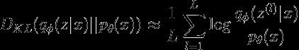
in which each z is sampled through
其中每个z通过
and see if the result is similar to the one you obtain with the analytical solution.
并查看结果是否与您通过分析解决方案获得的结果相似。
Lastly, if you don’t want to manually compute the KL divergence, you may use the function from TensorFlow Probability library, which directly computes the KL divergence between two distributions:
最后,如果您不想手动计算KL散度,则可以使用TensorFlow概率库中的函数,该函数直接计算两个分布之间的KL散度:
prior_dist = tfd.MultivariateNormalDiag(loc=tf.zeros((batch_size, latent_dim)), scale_diag=tf.ones((batch_size, latent_dim)))
var_post_dist = tfd.MultivariateNormalDiag(loc=mu, scale_diag=sd)
kl_divergence = tfd.kl_divergence(distribution_a=var_post_dist, distribution_b=prior_dist)
Now that we just mentioned TFP, it’s a good time to jump into the next version of implementation, which is all about this library.
既然我们刚刚提到了TFP,现在是进入下一个实现版本的好时机了,这与该库有关。
版本b。 (Version b.)
By combining TFP with Keras API of TF2, the code looks much simpler than the one in Version a. It is actually my favorite version, and will be the one I use in the future due to its simplicity.
通过将TFP与TF2的Keras API结合使用,该代码看起来比版本a中的代码简单得多。 它实际上是我最喜欢的版本,由于它的简单性,它将成为我将来使用的版本。
In this version, the output of both the encoder and the decoder are objects from tensorflow_probability.distributions module, which have many methods you’d expect from a probabilistic distribution: mean, mode, sample, prob, log_prob, etc. To obtain such output from encoder and decoder, you only need to replace their output layer with one of the tensorflow_probability.layers objects.
在此版本中,编码器和解码器的输出都是来自tensorflow_probability.distributions模块的对象, tensorflow_probability.distributions模块具有您希望从概率分布中获得的许多方法: mean , mode , sample , prob , log_prob等。要获取此类输出从编码器和解码器开始,您只需要用tensorflow_probability.layers对象之一替换其输出层tensorflow_probability.layers 。
The implementation is as follows:
实现如下:
class VAE_MNIST:

    def __init__(self, dim_z, kl_weight, learning_rate):
        self.dim_x = (28, 28, 1)
        self.dim_z = dim_z
        self.kl_weight = kl_weight
        self.learning_rate = learning_rate


    # Sequential API encoder
    def encoder_z(self):
        # define prior distribution for the code, which is an isotropic Gaussian
        prior = tfd.Independent(tfd.Normal(loc=tf.zeros(self.dim_z), scale=1.),
                                reinterpreted_batch_ndims=1)
        # build layers argument for tfk.Sequential()
        input_shape = self.dim_x
        layers = [tfkl.InputLayer(input_shape=input_shape)]
        layers.append(tfkl.Conv2D(filters=32, kernel_size=3, strides=(2,2),
                                  padding='valid', activation='relu'))
        layers.append(tfkl.Conv2D(filters=64, kernel_size=3, strides=(2,2),
                                  padding='valid', activation='relu'))
        layers.append(tfkl.Flatten())
        # the following two lines set the output to be a probabilistic distribution
        layers.append(tfkl.Dense(tfpl.IndependentNormal.params_size(self.dim_z),
                                 activation=None, name='z_params'))
        layers.append(tfpl.IndependentNormal(self.dim_z,
            convert_to_tensor_fn=tfd.Distribution.sample,
            activity_regularizer=tfpl.KLDivergenceRegularizer(prior, weight=self.kl_weight),
            name='z_layer'))
        return tfk.Sequential(layers, name='encoder')

    # Sequential API decoder
    def decoder_x(self):
        layers = [tfkl.InputLayer(input_shape=self.dim_z)]
        layers.append(tfkl.Dense(7*7*32, activation=None))
        layers.append(tfkl.Reshape((7,7,32)))
        layers.append(tfkl.Conv2DTranspose(filters=64, kernel_size=3, strides=2,
                                           padding='same', activation='relu'))
        layers.append(tfkl.Conv2DTranspose(filters=32, kernel_size=3, strides=2,
                                           padding='same', activation='relu'))
        layers.append(tfkl.Conv2DTranspose(filters=1, kernel_size=3, strides=1,
                                           padding='same'))
        layers.append(tfkl.Flatten(name='x_params'))
        # note that here we don't need
        # `tfkl.Dense(tfpl.IndependentBernoulli.params_size(self.dim_x))` because
        # we've restored the desired input shape with the last Conv2DTranspose layer
        layers.append(tfpl.IndependentBernoulli(self.dim_x, name='x_layer'))
        return tfk.Sequential(layers, name='decoder')

    def build_vae_keras_model(self):
        x_input = tfk.Input(shape=self.dim_x)
        encoder = self.encoder_z()
        decoder = self.decoder_x()
        z = encoder(x_input)


        # compile VAE model
        model = tfk.Model(inputs=x_input, outputs=decoder(z))
        model.compile(loss=negative_log_likelihood,
                      optimizer=tfk.optimizers.Adam(self.learning_rate))
        return model


# the negative of log-likelihood for probabilistic output
negative_log_likelihood = lambda x, rv_x: -rv_x.log_prob(x)
That’s it! 62 lines of code after code reformatting, including comments. One of the main reasons for such simplification is the sampling of z, as all of the steps of the reparameterization trick have been abstracted through the encoder output TFP layer tfpl.IndependentNormal. Furthermore, the KL divergence computation is done through the activity_regularizer argument in that probabilistic encoder output layer, where we specify the prior distribution to be the standard multivariate Gaussian distribution, as well as the KL divergence weight ω, to create a tfpl.KLDivergenceRegularizer object. In addition, the expected reconstruction error can be computed by simply calling the log_prob method of the decoder output, which is a tfp.distributions.Independent object — this is as neat as it can get.
而已! 重新格式化后的62行代码(包括注释)。 简化的主要原因之一是z的采样,因为重新参数化技巧的所有步骤都已通过编码器输出TFP层tfpl.IndependentNormal进行了抽象。 此外,KL散度计算是通过该概率编码器输出层中的activity_regularizer参数完成的,其中我们将先验分布指定为标准多元高斯分布,并指定KL散度权重ω ,以创建tfpl.KLDivergenceRegularizer对象。 此外,可以通过简单地调用解码器输出的log_prob方法来计算预期的重构误差,该方法是tfp.distributions.Independent对象-尽可能简洁。
One caveat is that one might think since the input to the decoder needs to be a tensor, but z is a tfp.distributions.Independent object (see Line 53), we need to instead write z = encoder(x_input).sample() to explicitly sample z. Doing so is not only unnecessary, but also incorrect:
一个警告是,由于解码器的输入需要是张量,而z是tfp.distributions.Independent对象(请参见第53行 ),因此我们可能需要写成z = encoder(x_input).sample()显式采样z 。 这样做不仅是不必要的,而且是不正确的:
unnecessary because we have
convert_to_tensor_fnset totfd.Distribution.sample(which is actually the default value but I wrote it out explicitly so you can see): what this argument does is that whenever the output of this layer is treated as atf.Tensorobject, like in our case when we need a sample from this distribution —outputs=decoder(z)in Line 56, it will call the method specified byconvert_to_tensor_fn, so it’s already doingoutputs=decoder(z.sample()).因为我们将
convert_to_tensor_fn设置为tfd.Distribution.sample(实际上是默认值,但是我将其明确写出,以便您可以看到),所以没有必要:此参数的作用是,只要将此层的输出视为tf.Tensor对象,就像我们需要从该分布中获取样本的情况一样outputs=decoder(z)第56行中的outputs=decoder(z.sample())outputs=decoder(z),它将调用由convert_to_tensor_fn指定的方法,因此它已经在执行outputs=decoder(z.sample())。incorrect because with
.sample()being explicitly called, the KL divergence, which is supposed to be computed bytfpl.KLDivergenceRegularizer, would not get picked up as part of the cost. It might be that after.sample()is called, we no longer have z as atfp.distributions.Independentobject in the computational graph of the neural network, which is the object type that containstfpl.KLDivergenceRegularizeras itsactivity_regularizer. Therefore, doing.sample()for the encoder output in this version of implementing VAE would give us a loss function that only contains the expected reconstruction error — the trained VAE would no longer serve as a generative model, but one that only reconstructs its input.这是不正确的,因为显式调用
.sample(),应该由tfpl.KLDivergenceRegularizer计算出的KL散度不会作为成本的一部分被tfpl.KLDivergenceRegularizer。 可能是因为在.sample()之后,我们在神经网络的计算图中不再拥有z作为tfp.distributions.Independent对象,该对象类型包含tfpl.KLDivergenceRegularizer作为activity_regularizer的对象类型。 因此,在此版本的实现VAE中对编码器输出执行.sample()会给我们带来一个损失函数,该函数仅包含预期的重构误差-受过训练的VAE将不再充当生成模型,而是仅重构其输入的模型。
This version of implementation is very similar to this tutorial by TensorFlow, which does a much better job than the one showed under Version a. — both reconstruction of existing digits and generation of new digits would work. Only a couple of things I want to address for this post:
该版本的实现与TensorFlow的本教程非常相似, 该教程比版本a中显示的教程做得更好。 —既可以重建现有数字又可以生成新数字。 我只想为这篇文章介绍几件事:
They applied
tfpl.MultivariateNormalTriLinstead oftfpl.IndependentNormalas the encoder output probabilistic layer, which essentially trains the non-zero elements of a lower triangular matrix that is conceptually derived from Cholesky decomposition of a positive definite matrix. Such positive definite matrix is essentially the covariance matrix of the posterior distribution of z, and can be any positive definite matrix, instead of just a diagonal matrix assumed in the VAE paper. This would give us a more flexible posterior distribution, but also contains more parameters to train, and the KL divergence is more complicated to compute.他们将
tfpl.MultivariateNormalTriL而不是tfpl.IndependentNormal用作编码器输出概率层,该层实质上训练了下三角矩阵的非零元素,该元素从概念上是从正定矩阵的Cholesky分解中得出的。 这样的正定矩阵本质上是z的后分布的协方差矩阵,并且可以是任何正定矩阵,而不仅仅是VAE论文中假设的对角矩阵。 这将为我们提供更灵活的后验分布,但还包含更多要训练的参数,并且KL散度的计算更加复杂。They set the KL divergence
weightas the default 1.0 intfpl.KLDivergenceRegularizer, but like I discussed under Part I, this hyperparameter is crucial to the success of a VAE implementation, and usually needs to be explicitly tuned to optimize the model performance.他们在
tfpl.KLDivergenceRegularizer中将KL散度weight设置为默认值1.0 ,但是正如我在第I部分中讨论的那样,此超参数对于VAE实现的成功至关重要,通常需要进行显式调整以优化模型性能。
Lastly for this implementation version, I want to show one perk of applying TFP layer as the decoder output: that we are able to obtain more flexible predictions. For the original VAE, the decoder output is deterministic, therefore after sampling z, the decoder output is set. However, with the output being a distribution, we can call mean, mode, or sample method to output a tf.Tensor object as the digit image prediction. Here are the results when different methods are called, for both reconstruction and generation:
最后,对于该实现版本,我想展示一个应用TFP层作为解码器输出的好处:我们能够获得更灵活的预测。 对于原始VAE,解码器输出是确定性的,因此在对z进行采样之后,将设置解码器输出。 但是,由于输出是分布,我们可以调用mean , mode或sample方法来输出tf.Tensor对象作为数字图像预测。 这是调用不同方法进行重构和生成时的结果:
Note that for both reconstruction and generation, the mean appears to be more blurry than (or not as sharp as) the mode, since the mean of a Bernoulli distribution is a value between 0 and 1, while the mode is either 0 (when parameter is less than 0.5) or 1 (otherwise); the sample shows more granularity than the other two while also looks sharp, since each pixel is a random sample (unlike the mode, which after training basically knows what values all pixels would take as a whole to form a digit) that also takes either 0 or 1 as its value. This is the flexibility that a probabilistic distribution can provide.
请注意,对于重建和生成,均值似乎比该模式更模糊(或不如该模式锐利),因为伯努利分布的均值为0到1之间的值,而该模式为0 (当参数为小于0.5 )或1 (否则); 该样本显示的粒度比其他两个样本都更细,同时看起来也很清晰,因为每个像素都是随机样本(与模式不同,该模式在训练后基本上知道所有像素将整体形成一个数字的值),该样本也取0或1作为其值。 这是概率分布可以提供的灵活性。
The following two versions of implementation focus on how to customize the loss function to compute the expected reconstruction error correctly while applying Keras API to simplify the code; since the discussion in Version a. already set the foundation for these two versions, I can focus mainly on demonstrate the code.
以下两个版本的实现侧重于如何应用Keras API简化代码时自定义损失函数以正确计算预期的重构误差; 自版本a中的讨论。 已经为这两个版本奠定了基础,我可以主要集中在演示代码上。
版本c。 (Version c.)
In Version a. we talked about how directly using tf.nn.sigmoid_cross_entropy_with_logits for the loss argument when compile the tfk.Model object would result in a incorrect computation of the expected reconstruction error; a quick fix is to implement a custom loss function based on tf.nn.sigmoid_cross_entropy_with_logits as follows:
在版本a中。 我们讨论了在compile tfk.Model对象时,如何直接使用tf.nn.sigmoid_cross_entropy_with_logits作为loss参数,这会导致错误地计算预期的重构错误; 一个快速的解决方案是基于tf.nn.sigmoid_cross_entropy_with_logits实现自定义损失函数,如下所示:
def custom_sigmoid_cross_entropy_loss_with_logits(x_true, x_recons_logits):
    raw_cross_entropy = tf.nn.sigmoid_cross_entropy_with_logits(
                                                      labels=x_true,
                                                      logits=x_recons_logits)
    neg_log_likelihood = tf.math.reduce_sum(raw_cross_entropy, axis=[1, 2, 3])
    return tf.math.reduce_mean(neg_log_likelihood)
in which we take the sum of the cross-entropy losses across all pixel dimensions for each instance. And when compiling the model, we write
其中,我们对每个实例取所有像素尺寸上的交叉熵损失之和。 在编译模型时,我们写
model.compile(loss=Note that the decoder is the same one as in Version a., which deterministically outputs the logits of parameters of the independent Bernoulli distribution. Meanwhile, we use tfpl.IndependentNormal as the encoder output layer just like in Version b., thus the KL divergence computation is taken care of by its argument activity_regularizer.
请注意,解码器与版本a中的解码器相同。 ,确定性地输出独立伯努利分布的参数对数。 同时,就像版本b中一样,我们使用tfpl.IndependentNormal作为编码器输出层。 因此,KL散度计算由其参数activity_regularizer 。
Similarly, we have the following implementation version:
同样,我们有以下实现版本:
版本d。 (Version d.)
We build another custom loss function upon tfk.losses.BinaryCrossentropy as follows:
We build another custom loss function upon tfk.losses.BinaryCrossentropy as follows:
def custom_binary_cross_entropy_loss(x_true, x_recons_dist):
    x_recons_mean = x_recons_dist.mean()
    raw_cross_entropy = tfk.losses.BinaryCrossentropy(
                reduction=tfk.losses.Reduction.NONE)(x_true, x_recons_mean)
    neg_log_likelihood = tf.math.reduce_sum(raw_cross_entropy, axis=[1, 2])
    return tf.math.reduce_mean(neg_log_likelihood)
Note that unlike Version c. which uses a deterministic decoder output layer, this version apples a probabilistic layer just like in Version b.; however, we need to take the mean of this distribution first (Line 2 of above code block), because one of the arguments for tfk.losses.BinaryCrossentropy object is the parameter of the Bernoulli distribution, which is the same as its mean. Also note the argument reduction when initializing the tfk.losses.BinaryCrossentropy object, which is set to tfk.losses.Reduction.NONE: this prevents the program from making further operations on the resulting tensor that is of the same shape as the mini-batch digit image tensor, each element of whose contains the cross-entropy loss for one specific pixel. We then take the sum over the dimensions at the instance level, just like what we did in the custom loss function in Version c.
Note that unlike Version c. which uses a deterministic decoder output layer, this version apples a probabilistic layer just like in Version b. ; however, we need to take the mean of this distribution first (Line 2 of above code block), because one of the arguments for tfk.losses.BinaryCrossentropy object is the parameter of the Bernoulli distribution, which is the same as its mean. Also note the argument reduction when initializing the tfk.losses.BinaryCrossentropy object, which is set to tfk.losses.Reduction.NONE : this prevents the program from making further operations on the resulting tensor that is of the same shape as the mini-batch digit image tensor, each element of whose contains the cross-entropy loss for one specific pixel. We then take the sum over the dimensions at the instance level, just like what we did in the custom loss function in Version c.
It’s worth pointing out that any function we define for the loss argument when compile the model must take exactly two arguments, with one being the data that the model tries to predict, and the other being the model output. Therefore, we’d have a problem whenever we want to apply Keras API while having a more flexible loss function. We are lucky to have the activity_regularizer argument in the encoder output TFP layer that helps incorporate the KL divergence into the computation of cost, which gives us Version b.; but what if we don’t? The remaining two versions introduces a way to implement a more flexible loss function in general, not just for the specific case of VAE — thanks to add_loss method of tfkl.Layer class.
It's worth pointing out that any function we define for the loss argument when compile the model must take exactly two arguments, with one being the data that the model tries to predict, and the other being the model output. Therefore, we'd have a problem whenever we want to apply Keras API while having a more flexible loss function. We are lucky to have the activity_regularizer argument in the encoder output TFP layer that helps incorporate the KL divergence into the computation of cost, which gives us Version b. ; but what if we don't? The remaining two versions introduces a way to implement a more flexible loss function in general, not just for the specific case of VAE — thanks to add_loss method of tfkl.Layer class.
Version e. (Version e.)
I will start by directly demonstrate the code for this version:
I will start by directly demonstrate the code for this version:
class VAE_MNIST(tfk.Model):

    def __init__(self, dim_z, kl_weight=1, name="autoencoder", **kwargs):
        super(VAE_MNIST, self).__init__(name=name, **kwargs)
        self.dim_x = (28, 28, 1)
        self.dim_z = dim_z
        self.encoder = self.encoder_z()
        self.decoder = self.decoder_x()
        self.kl_weight = kl_weight

    # Sequential API encoder
    def encoder_z(self):
        layers = [tfkl.InputLayer(input_shape=self.dim_x)]
        layers.append(tfkl.Conv2D(filters=32, kernel_size=3, strides=(2,2),
                                  padding='valid', activation='relu'))
        layers.append(tfkl.Conv2D(filters=64, kernel_size=3, strides=(2,2),
                                  padding='valid', activation='relu'))
        layers.append(tfkl.Flatten())
        # *2 because number of parameters for both mean and (raw) standard deviation
        layers.append(tfkl.Dense(self.dim_z*2, activation=None))
        return tfk.Sequential(layers)

    def encode(self, x_input):
        mu, rho = tf.split(self.encoder(x_input), num_or_size_splits=2, axis=1)
        sd = tf.math.log(1+tf.math.exp(rho))
        z_sample = mu + sd * tf.random.normal(shape=(self.dim_z,))
        return z_sample, mu, sd

    # Sequential API decoder
    def decoder_x(self):
        layers = [tfkl.InputLayer(input_shape=self.dim_z)]
        layers.append(tfkl.Dense(7*7*32, activation=None))
        layers.append(tfkl.Reshape((7,7,32)))
        layers.append(tfkl.Conv2DTranspose(filters=64, kernel_size=3, strides=2,
                                           padding='same', activation='relu'))
        layers.append(tfkl.Conv2DTranspose(filters=32, kernel_size=3, strides=2,
                                           padding='same', activation='relu'))
        layers.append(tfkl.Conv2DTranspose(filters=1, kernel_size=3, strides=1,
                                           padding='same'))
        return tfk.Sequential(layers, name='decoder')

    def call(self, x_input):
        z_sample, mu, sd = self.encode(x_input)
        kl_divergence = tf.math.reduce_mean(- 0.5 *
                tf.math.reduce_sum(1+tf.math.log(
                tf.math.square(sd))-tf.math.square(mu)-tf.math.square(sd), axis=1))
        x_logits = self.decoder(z_sample)
        # VAE_MNIST is inherited from tfk.Model, thus have class method add_loss()
        self.add_loss(self.kl_weight * kl_divergence)
        return x_logits

# custom loss function with tf.nn.sigmoid_cross_entropy_with_logits
def custom_sigmoid_cross_entropy_loss_with_logits(x_true, x_recons_logits):
    raw_cross_entropy = tf.nn.sigmoid_cross_entropy_with_logits(
                                            labels=x_true, logits=x_recons_logits)
    neg_log_likelihood = tf.math.reduce_sum(raw_cross_entropy, axis=[1, 2, 3])
    return tf.math.reduce_mean(neg_log_likelihood)


####################   The following code shows how to train the model   ####################
# set hyperparameters
epochs = 10
batch_size = 32
lr = 0.0001
latent_dim=16
kl_w=3
# compile and train tfk.Model
vae = VAE_MNIST(dim_z=latent_dim, kl_weight=kl_w)
vae.compile(optimizer=tf.keras.optimizers.Adam(learning_rate=lr),
            loss=custom_sigmoid_cross_entropy_loss_with_logits)
train_history = vae.fit(x=train_images, y=train_images, batch_size=batch_size, epochs=epochs,
                        verbose=1, validation_data=(test_images, test_images), shuffle=True)
Note that I used the exact same loss function as the one in Version c. when compile the tfk.Model (Line 70). The weighted KL divergence is incorporated into the computation of the cost through calling the add_loss class method (Line 49). The following is a direct quote from its documentation:
Note that I used the exact same loss function as the one in Version c. when compile the tfk.Model (Line 70 ). The weighted KL divergence is incorporated into the computation of the cost through calling the add_loss class method (Line 49 ). The following is a direct quote from its documentation :
This method can be used inside a subclassed layer or model’s
callfunction, in which caselossesshould be a Tensor or list of Tensors.This method can be used inside a subclassed layer or model's
callfunction, in which caselossesshould be a Tensor or list of Tensors.
Without any requirements to the format besides being “a Tensor or list of Tensors”, we can build a much more flexible loss function. The tricky part comes from the first half of that quote, which specifies where this method shall be called: note that in my implementation, I called it inside the call function of VAE_MNIST class, which inherits from tfk.Model class. This is different from implementation Version b., which doesn’t have class inheritance. For this version, I originally also started by writing VAE_MNIST class with no class inheritance, and call compile method for the tfk.Model object in the class function named build_vae_keras_model, just like what I did in Version b. After the tfk.Model object model gets compiled, I directly called model.add_loss(self.kl_weight * kl_divergence) — my rationale is that since the output layer of our model, an object of class tfkl.Conv2DTranspose, inherits from tfkl.Layer, we shall be able to conduct such operation. However, the training result is that I’d get “brighter” generated image if I turn the KL weight down, to around 0.01; and if I start to increase KL weight, I’d get almost completely dark generated images. Overall, the generated images would have poor quality, while the reconstructed images would look great but wouldn’t change at all with different values of KL weight. Only after I inherited VAE_MNIST from tfk.Model class, and changed the name of the class method where add_loss gets called to call, would the model train properly.
Without any requirements to the format besides being “a Tensor or list of Tensors”, we can build a much more flexible loss function. The tricky part comes from the first half of that quote, which specifies where this method shall be called: note that in my implementation, I called it inside the call function of VAE_MNIST class, which inherits from tfk.Model class. This is different from implementation Version b. , which doesn't have class inheritance. For this version, I originally also started by writing VAE_MNIST class with no class inheritance, and call compile method for the tfk.Model object in the class function named build_vae_keras_model , just like what I did in Version b. After the tfk.Model object model gets compiled, I directly called model.add_loss(self.kl_weight * kl_divergence) — my rationale is that since the output layer of our model, an object of class tfkl.Conv2DTranspose , inherits from tfkl.Layer , we shall be able to conduct such operation. However, the training result is that I'd get “brighter” generated image if I turn the KL weight down, to around 0.01 ; and if I start to increase KL weight, I'd get almost completely dark generated images. Overall, the generated images would have poor quality, while the reconstructed images would look great but wouldn't change at all with different values of KL weight. Only after I inherited VAE_MNIST from tfk.Model class, and changed the name of the class method where add_loss gets called to call , would the model train properly.
Version f.
Version f.
I implemented this version as the last one for practice, imagining that such framework might come in handy if one day I need to implement some model that’s too complicated to use Keras API. Here’s the code:
I implemented this version as the last one for practice, imagining that such framework might come in handy if one day I need to implement some model that's too complicated to use Keras API. 这是代码:
class Sampler_Z(tfk.layers.Layer):

    def call(self, inputs):
        mu, rho = inputs
        sd = tf.math.log(1+tf.math.exp(rho))
        batch_size = tf.shape(mu)[0]
        dim_z = tf.shape(mu)[1]
        z_sample = mu + sd * tf.random.normal(shape=(batch_size, dim_z))
        return z_sample, sd


class Encoder_Z(tfk.layers.Layer):

    def __init__(self, dim_z, name="encoder", **kwargs):
        super(Encoder_Z, self).__init__(name=name, **kwargs)
        self.dim_x = (28, 28, 1)
        self.dim_z = dim_z
        self.conv_layer_1 = tfkl.Conv2D(filters=32, kernel_size=3, strides=(2,2),
                                        padding='valid', activation='relu')
        self.conv_layer_2 = tfkl.Conv2D(filters=64, kernel_size=3, strides=(2,2),
                                        padding='valid', activation='relu')
        self.flatten_layer = tfkl.Flatten()
        self.dense_mean = tfkl.Dense(self.dim_z, activation=None, name='z_mean')
        self.dense_raw_stddev = tfkl.Dense(self.dim_z, activation=None, name='z_raw_stddev')
        self.sampler_z = Sampler_Z()

    # Functional
    def call(self, x_input):
        z = self.conv_layer_1(x_input)
        z = self.conv_layer_2(z)
        z = self.flatten_layer(z)
        mu = self.dense_mean(z)
        rho = self.dense_raw_stddev(z)
        z_sample, sd = self.sampler_z((mu,rho))
        return z_sample, mu, sd

class Decoder_X(tfk.layers.Layer):

    def __init__(self, dim_z, name="decoder", **kwargs):
        super(Decoder_X, self).__init__(name=name, **kwargs)
        self.dim_z = dim_z
        self.dense_z_input = tfkl.Dense(7*7*32, activation=None)
        self.reshape_layer = tfkl.Reshape((7,7,32))
        self.conv_transpose_layer_1 = tfkl.Conv2DTranspose(filters=64, kernel_size=3, strides=2,
                                                           padding='same', activation='relu')
        self.conv_transpose_layer_2 = tfkl.Conv2DTranspose(filters=32, kernel_size=3, strides=2,
                                                           padding='same', activation='relu')
        self.conv_transpose_layer_3 = tfkl.Conv2DTranspose(filters=1, kernel_size=3, strides=1,
                                                           padding='same')

    # Functional
    def call(self, z):
        x_output = self.dense_z_input(z)
        x_output = self.reshape_layer(x_output)
        x_output = self.conv_transpose_layer_1(x_output)
        x_output = self.conv_transpose_layer_2(x_output)
        x_output = self.conv_transpose_layer_3(x_output)
        return x_output

class VAE_MNIST(tfk.Model):

    def __init__(self, dim_z, learning_rate, kl_weight=1, name="autoencoder", **kwargs):
        super(VAE_MNIST, self).__init__(name=name, **kwargs)
        self.dim_x = (28, 28, 1)
        self.dim_z = dim_z
        self.learning_rate = learning_rate
        self.encoder = Encoder_Z(dim_z=self.dim_z)
        self.decoder = Decoder_X(dim_z=self.dim_z)
        self.kl_weight = kl_weight

    # def encode_and_decode(self, x_input):
    def call(self, x_input):
        z_sample, mu, sd = self.encoder(x_input)
        x_recons_logits = self.decoder(z_sample)

        kl_divergence = - 0.5 * tf.math.reduce_sum(1+tf.math.log(
          tf.math.square(sd))-tf.math.square(mu)-tf.math.square(sd), axis=1)
        kl_divergence = tf.math.reduce_mean(kl_divergence)
        # self.add_loss(lambda: self.kl_weight * kl_divergence)
        self.add_loss(self.kl_weight * kl_divergence)
        return x_recons_logits


# vae loss function -- only the negative log-likelihood part,
# since we use add_loss for the KL divergence part
def partial_vae_loss(x_true, model):
    # x_recons_logits = model.encode_and_decode(x_true)
    x_recons_logits = model(x_true)
    # compute cross entropy loss for each dimension of every datapoint
    raw_cross_entropy = tf.nn.sigmoid_cross_entropy_with_logits(
      labels=x_true, logits=x_recons_logits)
    neg_log_likelihood = tf.math.reduce_sum(raw_cross_entropy, axis=[1, 2, 3])
    return tf.math.reduce_mean(neg_log_likelihood)


@tf.function
def train_step(x_true, model, optimizer, loss_metric):
    with tf.GradientTape() as tape:
        neg_log_lik = partial_vae_loss(x_true, model)
        # kl_loss = model.losses[-1]
        kl_loss = tf.math.reduce_sum(model.losses)  # vae.losses is a list
        total_vae_loss = neg_log_lik + kl_loss
    gradients = tape.gradient(total_vae_loss, model.trainable_variables)
    optimizer.apply_gradients(zip(gradients, model.trainable_variables))
    loss_metric(total_vae_loss)

####################   The following code shows how to train the model   ####################
# set hyperparameters
train_size = 60000
batch_size = 64
test_size = 10000
latent_dim=16
lr = 0.0005
kl_w = 3
epochs = 10
num_examples_to_generate = 16
train_dataset = (tf.data.Dataset.from_tensor_slices(train_images)
                 .shuffle(train_size).batch(batch_size))
test_dataset = (tf.data.Dataset.from_tensor_slices(test_images)
                .shuffle(test_size).batch(batch_size))
# model training
vae = VAE_MNIST(dim_z=latent_dim, learning_rate=lr, analytic_kl=True, kl_weight=kl_w)
loss_metric = tf.keras.metrics.Mean()
opt = tfk.optimizers.Adam(vae.learning_rate)


for epoch in range(epochs):
    start_time = time.time()
    for train_x in tqdm(train_dataset):
        train_step(train_x, vae, opt, loss_metric)
    end_time = time.time()
    elbo = -loss_metric.result()
    #display.clear_output(wait=False)
    print('Epoch: {}, Train set ELBO: {}, time elapse for current epoch: {}'.format(
            epoch, elbo, end_time - start_time))
    generate_images(vae, test_sample)
I want to emphasize on the importance of naming the class method that calls the add_loss method as call: notice that this method was named encode_and_decode originally (Line 70) — if I add @tf.function decorator for train_step method (Line 94) before renaming the class method, I’d get
I want to emphasize on the importance of naming the class method that calls the add_loss method as call : notice that this method was named encode_and_decode originally (Line 70 ) — if I add @tf.function decorator for train_step method (Line 94 ) before renaming the class method, I'd get
TypeError: An op outside of the function building code is being passed a “Graph” tensor. It is possible to have Graph tensors leak out of the function building context by including a tf.init_scope in your function building code.After I modified the class method name accordingly, the error disappeared. It’s important to have the @tf.function decorator because it significantly improves the training speed: before renaming, the last epoch ran for 1041 seconds (and the time lapse for each epoch increased from epoch to epoch; the first epoch “only” ran for 139 seconds, which is another strange phenomenon); after renaming, every epoch has running time between 34.7 seconds and 39.4 seconds.
After I modified the class method name accordingly, the error disappeared. It's important to have the @tf.function decorator because it significantly improves the training speed: before renaming, the last epoch ran for 1041 seconds (and the time lapse for each epoch increased from epoch to epoch; the first epoch “only” ran for 139 seconds, which is another strange phenomenon); after renaming, every epoch has running time between 34.7 seconds and 39.4 seconds.
Moreover, before renaming, I’d need to add the lambda argument for add_loss method (Line 78), since without lambda: I’d get the following error:
Moreover, before renaming, I'd need to add the lambda argument for add_loss method (Line 78 ), since without lambda: I'd get the following error:
ValueError: Expected a symbolic Tensors or a callable for the loss value. Please wrap your loss computation in a zero argument lambda.In short, when you plan to apply add_loss method to implement a more flexible loss function, a good practice is to subclass the tfk.Model class, and call the add_loss method inside a class method named call.
In short, when you plan to apply add_loss method to implement a more flexible loss function, a good practice is to subclass the tfk.Model class, and call the add_loss method inside a class method named call .
结论 (Conclusion)
In this post, I presented 6 different ways of implementing the VAE model that trains on the MNIST dataset, and gave a detailed review on VAE from a practical standpoint. In general, I would recommend a first-time VAE implementer to start with Version a., and then try to apply Keras API to simplify the code, with custom loss function to compute the expected reconstruction error just like Version c. and Version d.; after gaining a decent understanding of the model, it would be nice to adopt Version b., which is the most concise and IMHO the most elegant version. If one wants to prepare for implementing a very flexible loss function in general in the future, Version e. or Version f. could be a good place to start.
In this post, I presented 6 different ways of implementing the VAE model that trains on the MNIST dataset, and gave a detailed review on VAE from a practical standpoint. In general, I would recommend a first-time VAE implementer to start with Version a. , and then try to apply Keras API to simplify the code, with custom loss function to compute the expected reconstruction error just like Version c. and Version d. ; after gaining a decent understanding of the model, it would be nice to adopt Version b. , which is the most concise and IMHO the most elegant version. If one wants to prepare for implementing a very flexible loss function in general in the future, Version e. or Version f. could be a good place to start.
翻译自: https://towardsdatascience.com/6-different-ways-of-implementing-vae-with-tensorflow-2-and-tensorflow-probability-9fe34a8ab981
vae 实现