Antiderivative
In calculus, an antiderivative, inverse derivative, primitive function, primitive integral or indefinite integral[Note 1] of a function f is a differentiable function F whose derivative is equal to the original function f. This can be stated symbolically as F’ = f.[1][2] The process of solving for antiderivatives is called antidifferentiation (or indefinite integration), and its opposite operation is called differentiation, which is the process of finding a derivative. Antiderivatives are often denoted by capital Roman letters such as F and G.
Antiderivatives are related to definite integrals through the second fundamental theorem of calculus: the definite integral of a function over a closed interval where the function is Riemann integrable is equal to the difference between the values of an antiderivative evaluated at the endpoints of the interval.
In physics, antiderivatives arise in the context of rectilinear motion (e.g., in explaining the relationship between position, velocity and acceleration).[3] The discrete equivalent of the notion of antiderivative is antidifference.
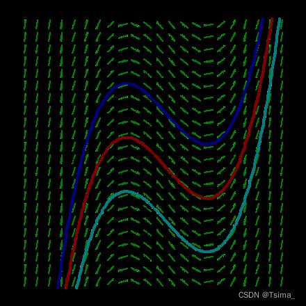
The slope field of {\displaystyle F(x)={\frac {x^{3}}{3}}-{\frac {x^{2}}{2}}-x+c}{\displaystyle F(x)={\frac {x^{3}}{3}}-{\frac {x^{2}}{2}}-x+c}, showing three of the infinitely many solutions that can be produced by varying the arbitrary constant c.
Contents
- 1 Examples
- 2 Uses and properties
- 3 Techniques of integration
- 4 Of non-continuous functions
-
- 4.1 Some examples
- 5 Basic formulae
- 6 See also
1 Examples
The function {\displaystyle F(x)={\tfrac {x^{3}}{3}}}{\displaystyle F(x)={\tfrac {x^{3}}{3}}} is an antiderivative of {\displaystyle f(x)=x{2}}f(x)=x{2}, since the derivative of {\displaystyle {\tfrac {x^{3}}{3}}}{\displaystyle {\tfrac {x^{3}}{3}}} is {\displaystyle x{2}}x{2}, and since the derivative of a constant is zero, {\displaystyle x{2}}x{2} will have an infinite number of antiderivatives, such as {\displaystyle {\tfrac {x^{3}}{3}},{\tfrac {x^{3}}{3}}+1,{\tfrac {x^{3}}{3}}-2}{\displaystyle {\tfrac {x^{3}}{3}},{\tfrac {x^{3}}{3}}+1,{\tfrac {x^{3}}{3}}-2}, etc. Thus, all the antiderivatives of {\displaystyle x{2}}x{2} can be obtained by changing the value of c in {\displaystyle F(x)={\tfrac {x^{3}}{3}}+c}{\displaystyle F(x)={\tfrac {x^{3}}{3}}+c}, where c is an arbitrary constant known as the constant of integration. Essentially, the graphs of antiderivatives of a given function are vertical translations of each other, with each graph’s vertical location depending upon the value c.
More generally, the power function {\displaystyle f(x)=x{n}}f(x)=x{n} has antiderivative {\displaystyle F(x)={\tfrac {x^{n+1}}{n+1}}+c}{\displaystyle F(x)={\tfrac {x^{n+1}}{n+1}}+c} if n ≠ −1, and {\displaystyle F(x)=\ln |x|+c}{\displaystyle F(x)=\ln |x|+c} if n = −1.
In physics, the integration of acceleration yields velocity plus a constant. The constant is the initial velocity term that would be lost upon taking the derivative of velocity, because the derivative of a constant term is zero. This same pattern applies to further integrations and derivatives of motion (position, velocity, acceleration, and so on).[3] Thus, integration produces the relations of acceleration, velocity and displacement:
{\displaystyle \int a\ \mathrm {d} t=v+C}{\displaystyle \int a\ \mathrm {d} t=v+C}
{\displaystyle \int v\ \mathrm {d} t=d+C}{\displaystyle \int v\ \mathrm {d} t=d+C}