tensorflow2.0学习笔记（四）

数据加载

读取MNIST数据集，直接从tensorflow.keras里读取，代码：

import tensorflow as tf
from tensorflow import keras

# 读取数据集
(x, y), (x_test, y_test) = keras.datasets.mnist.load_data()
# 查看训练数据x,y的形状
print(x.shape)
print(y.shape)
# 查看x的数据范围
print(x.min(), x.max(), x.mean())
# 查看测试数据的范围
print(x_test.shape, y_test.shape)
# 对测试标签one-hot处理
y_onehot = tf.one_hot(y, depth=10)
print(y[:4])
print(y_onehot[:4])

(60000, 28, 28)
(60000,)
0 255 33.318421449829934
(10000, 28, 28) (10000,)
[5 0 4 1]
tf.Tensor(
[[0. 0. 0. 0. 0. 1. 0. 0. 0. 0.]
 [1. 0. 0. 0. 0. 0. 0. 0. 0. 0.]
 [0. 0. 0. 0. 1. 0. 0. 0. 0. 0.]
 [0. 1. 0. 0. 0. 0. 0. 0. 0. 0.]], shape=(4, 10), dtype=float32)

读取CIFAR10/100数据集（代码里有注释）：

import tensorflow as tf
from tensorflow import keras

(x, y), (x_test, y_test) = keras.datasets.cifar10.load_data()
print(x.shape, y.shape, x_test.shape, y_test.shape)
'''
结果：
(50000, 32, 32, 3) (50000, 1) (10000, 32, 32, 3) (10000, 1)
'''

# 查看x范围，y的范围
print(x.min(), x.max())
print(y.min(), y.max())
'''
结果：
0 255
0 9
'''

# 转换为tensor格式
db = tf.data.Dataset.from_tensor_slices((x_test, y_test))
print(db)
'''
结果：

'''

# 打乱数据
db = db.shuffle(10000)


# 数据预处理
def preprocess(x, y):
    x = tf.cast(x, dtype=tf.float32) / 255.
    y = tf.cast(y, dtype=tf.int32)
    y = tf.one_hot(y, depth=10)
    return x, y


db2 = db.map(preprocess)
res = next(iter(db2))
print(res[0].shape, res[1].shape)
'''
结果：
(32, 32, 3) (1, 10)
'''

# 批处理
db3 = db2.batch(32)
res = next(iter(db3))
print(res[0].shape, res[1].shape)
'''
结果：
(32, 32, 32, 3) (32, 1, 10)
'''

全连接

可以看看tf.keras.layers.Dense的参数

import tensorflow as tf
from tensorflow import keras

x = tf.random.normal([2, 3])

# 定义模型结构
model = keras.Sequential([
    keras.layers.Dense(2, activation='relu'),
    keras.layers.Dense(2, activation='relu'),
    keras.layers.Dense(2)
])

# 查看模型
model.build(input_shape=[None, 3])
model.summary()

# 查看每层的权重和偏置
for p in model.trainable_variables:
    print(p.name, p.shape)

Model: "sequential"
_________________________________________________________________
Layer (type)                 Output Shape              Param #   
=================================================================
dense (Dense)                multiple                  8         
_________________________________________________________________
dense_1 (Dense)              multiple                  6         
_________________________________________________________________
dense_2 (Dense)              multiple                  6         
=================================================================
Total params: 20
Trainable params: 20
Non-trainable params: 0
_________________________________________________________________
dense/kernel:0 (3, 2)
dense/bias:0 (2,)
dense_1/kernel:0 (2, 2)
dense_1/bias:0 (2,)
dense_2/kernel:0 (2, 2)
dense_2/bias:0 (2,)

误差计算

根据公式

import tensorflow as tf

y = tf.constant([1, 2, 3, 0, 2])
'''
tf.Tensor([1 2 3 0 2], shape=(5,), dtype=int32)
'''

y = tf.one_hot(y, depth=4)
'''
tf.Tensor(
[[0. 1. 0. 0.]
 [0. 0. 1. 0.]
 [0. 0. 0. 1.]
 [1. 0. 0. 0.]
 [0. 0. 1. 0.]], shape=(5, 4), dtype=float32)
'''

y = tf.cast(y, dtype=tf.float32)
'''
tf.Tensor(
[[0. 1. 0. 0.]
 [0. 0. 1. 0.]
 [0. 0. 0. 1.]
 [1. 0. 0. 0.]
 [0. 0. 1. 0.]], shape=(5, 4), dtype=float32)
'''

out = tf.random.normal([5, 4])

loss1 = tf.reduce_mean(tf.square(y - out))

loss2 = tf.square(tf.norm(y - out)) / (5 * 4)

loss3 = tf.reduce_mean(tf.losses.MSE(y, out))

print(loss1)
print(loss2)
print(loss3)
'''
tf.Tensor(1.0575342, shape=(), dtype=float32)
tf.Tensor(1.0575341, shape=(), dtype=float32)
tf.Tensor(1.0575342, shape=(), dtype=float32)
'''

'''
交叉熵计算
'''
a = tf.losses.categorical_crossentropy([0, 1, 0, 0], [0.01, 0.97, 0.01, 0.01])
b = tf.losses.categorical_crossentropy([0, 1, 0, 0], [0.97, 0.01, 0.01, 0.01])
print(a)
print(b)
'''
a = tf.Tensor(0.030459179, shape=(), dtype=float32)
b = tf.Tensor(4.6051702, shape=(), dtype=float32)
值越小，预测的越准确
'''

'''
做交叉熵前肯定要做个softmax，但tf里一般这么做
'''
x = tf.random.normal([1, 784])
y = tf.random.normal([784, 2])
b = tf.zeros([2])

logits = x @ y + b
out = tf.losses.categorical_crossentropy([[0, 1]], logits, from_logits=True)
print(out)
'''
out = tf.Tensor([8.848387], shape=(1,), dtype=float32)
'''

sigmoid + MSE 容易导致梯度消失或者爆炸，而且收敛也比较缓慢，但也不全是，在meta-learning中MSE表现比交叉熵好。

导数

利用tf进行二阶求导

import tensorflow as tf

w = tf.Variable(1.0)
b = tf.Variable(2.0)
x = tf.Variable(3.0)

# 二次求导
with tf.GradientTape() as t1:
    with tf.GradientTape() as t2:
        y = x * w + b
    dy_dw, dy_db = t2.gradient(y, [w, b])
d2y_dw2 = t1.gradient(dy_dw, w)

print(dy_dw)
print(dy_db)
print(d2y_dw2)
'''
dy_dw = tf.Tensor(3.0, shape=(), dtype=float32)
dy_db = tf.Tensor(1.0, shape=(), dtype=float32)
d2y_dw2 = None
'''

交叉熵

用tf实现交叉熵的函数

import tensorflow as tf

# 固定随机数
tf.random.set_seed(4323)

x = tf.random.normal([2, 4])

w = tf.random.normal([4, 3])

b = tf.zeros([3])

y = tf.constant([2, 0])

with tf.GradientTape() as tape:
    # watch的作用是指定观察对象
    tape.watch([w, b])
    logits = (x @ w + b)
    '''
    tf.reduce_mean 函数用于计算张量tensor沿着指定的数轴（tensor的某一维度）上的的平均值，
    主要用作降维或者计算tensor（图像）的平均值。
    
    tf.losses.categorical_crossentropy,交叉熵,
    当交叉熵等于0时达到最佳状态，也即是预测值与真实值完全吻合。
    
    tf.one_hot(),设置两个参数，一个实际值，一个depth，depth根据最后输出的个数决定
    
    from_logits=True,自动做softmax操作
    '''
    loss = tf.reduce_mean(tf.losses.categorical_crossentropy(tf.one_hot(y, depth=3), logits, from_logits=True))

grads = tape.gradient(loss, [w, b])
print('w grad:', grads[0])
'''
w grad: tf.Tensor(
[[-0.13532364  0.1658054  -0.03048175]
 [ 0.15821853  0.23038033 -0.3885989 ]
 [-0.78006303  0.68287045  0.09719262]
 [ 0.52645856 -0.42982587 -0.0966327 ]], shape=(4, 3), dtype=float32)
'''

print('b grad:', grads[1])
'''
b grad: tf.Tensor([-0.4103608   0.485506   -0.07514517], shape=(3,), dtype=float32)
'''

均方差

import tensorflow as tf

x = tf.random.normal([1, 3])
w = tf.ones([3, 2])
b = tf.ones([2])
y = tf.constant([0, 1])

with tf.GradientTape() as tape:
    tape.watch([w, b])
    logits = tf.sigmoid(x @ w + b)
    loss = tf.reduce_mean(tf.losses.MSE(y, logits))

grads = tape.gradient(loss, [w, b])
print('w grad:', grads[0])
'''
w grad: tf.Tensor(
[[-0.00957194  0.00275196]
 [-0.04200966  0.01207792]
 [ 0.08479026 -0.02437749]], shape=(3, 2), dtype=float32)
'''
print('b grad:', grads[1])
'''
b grad: tf.Tensor([ 0.13470937 -0.0387294 ], shape=(2,), dtype=float32)
'''

链式法则

import tensorflow as tf

x = tf.constant(1.)
w1 = tf.constant(2.)
b1 = tf.constant(1.)
w2 = tf.constant(2.)
b2 = tf.constant(1.)

with tf.GradientTape(persistent=True) as tape:
    tape.watch([w1, b1, w2, b2])

    y1 = x * w1 + b1
    y2 = y1 * w2 + b2

dy2_dy1 = tape.gradient(y2, [y1])[0]
dy1_dw1 = tape.gradient(y1, [w1])[0]
dy2_dw1 = tape.gradient(y2, [w1])[0]

print(dy2_dy1 * dy1_dw1)
print(dy2_dw1)
'''
tf.Tensor(2.0, shape=(), dtype=float32)
tf.Tensor(2.0, shape=(), dtype=float32)
'''

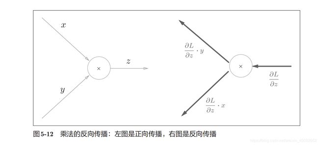
反向传播

FashionMNIST

FashionMNIST 是一个替代 MNIST 手写数字集的图像数据集。 它是由 Zalando（一家德国的时尚科技公司）旗下的研究部门提供。其涵盖了来自 10 种类别的共 7 万个不同商品的正面图片。FashionMNIST 的大小、格式和训练集 / 测试集划分与原始的 MNIST 完全一致。60000/10000 的训练测试数据划分，28x28 的灰度图片。
制作这个数据集的目的就是取代MNIST，作为机器学习算法良好的“检测器”，用以评估各种机器学习算法。为什么不用MNIST了呢？ 因为MNIST就现在的机器学习算法来说，是比较好分的，很多机器学习算法轻轻松松可以达到99%，因此无法区分出各类机器学习算法的优劣。
为了和MNIST兼容，Fashion-MNIST 与MNIST的格式，类别，数据量，train和test的划分，完全一致。

import tensorflow as tf
from tensorflow import keras
from tensorflow.keras import datasets, layers, optimizers, Sequential, metrics

import os

os.environ['TF_CPP_MIN_LOG_LEVEL'] = '2'


def preprocess(x, y):
    x = tf.cast(x, dtype=tf.float32) / 255.
    y = tf.cast(y, dtype=tf.int32)
    return x, y


(x, y), (x_test, y_test) = datasets.fashion_mnist.load_data()
print(x.shape, y.shape)

batchsz = 128

db = tf.data.Dataset.from_tensor_slices((x, y))
db = db.map(preprocess).shuffle(10000).batch(batchsz)

db_test = tf.data.Dataset.from_tensor_slices((x_test, y_test))
db_test = db_test.map(preprocess).batch(batchsz)

db_iter = iter(db)
sample = next(db_iter)
print('batch:', sample[0].shape, sample[1].shape)

model = Sequential([
    layers.Dense(256, activation=tf.nn.relu),  # [b, 784] => [b, 256]
    layers.Dense(128, activation=tf.nn.relu),  # [b, 256] => [b, 128]
    layers.Dense(64, activation=tf.nn.relu),  # [b, 128] => [b, 64]
    layers.Dense(32, activation=tf.nn.relu),  # [b, 64] => [b, 32]
    layers.Dense(10)  # [b, 32] => [b, 10], 330 = 32*10 + 10
])
model.build(input_shape=[None, 28 * 28])
model.summary()
# w = w - lr*grad
optimizer = optimizers.Adam(lr=1e-3)


def main():
    for epoch in range(30):

        for step, (x, y) in enumerate(db):

            # x: [b, 28, 28] => [b, 784]
            # y: [b]
            x = tf.reshape(x, [-1, 28 * 28])

            with tf.GradientTape() as tape:
                # [b, 784] => [b, 10]
                logits = model(x)
                y_onehot = tf.one_hot(y, depth=10)
                # [b]
                loss_mse = tf.reduce_mean(tf.losses.MSE(y_onehot, logits))
                loss_ce = tf.losses.categorical_crossentropy(y_onehot, logits, from_logits=True)
                loss_ce = tf.reduce_mean(loss_ce)

            grads = tape.gradient(loss_ce, model.trainable_variables)
            # 更新网络参数，w '= w - lr * grad
            optimizer.apply_gradients(zip(grads, model.trainable_variables))

            if step % 100 == 0:
                print(epoch, step, 'loss:', float(loss_ce), float(loss_mse))

        # test
        total_correct = 0
        total_num = 0
        for x, y in db_test:
            # x: [b, 28, 28] => [b, 784]
            # y: [b]
            x = tf.reshape(x, [-1, 28 * 28])
            # [b, 10]
            logits = model(x)
            # logits => prob, [b, 10]
            prob = tf.nn.softmax(logits, axis=1)
            # [b, 10] => [b], int64
            pred = tf.argmax(prob, axis=1)
            pred = tf.cast(pred, dtype=tf.int32)
            # pred:[b]
            # y: [b]
            # correct: [b], True: equal, False: not equal
            correct = tf.equal(pred, y)
            correct = tf.reduce_sum(tf.cast(correct, dtype=tf.int32))

            total_correct += int(correct)
            total_num += x.shape[0]

        acc = total_correct / total_num
        print(epoch, 'test acc:', acc)


if __name__ == '__main__':
    main()

29 0 loss: 0.07586537301540375 204.44126892089844
29 100 loss: 0.12027563899755478 173.48133850097656
29 200 loss: 0.05436631292104721 192.68887329101562
29 300 loss: 0.1850580871105194 157.16915893554688
29 400 loss: 0.05077245831489563 221.9516143798828
29 test acc: 0.8871

精度不高的原因是使用的是fashionMNIST数据集，难度肯定大些。

可视化

tensorboard这个工具进行可视化。
它工作的原则是：
1、监听路径
2、生成结构实例
3、把数据喂进结构里

首先进入conda虚拟环境，然后输入命令：

tensorboard --logdir logs

在浏览器里输入：

http://localhost:6006/

例子代码：

import tensorflow as tf
from tensorflow.keras import datasets, layers, optimizers, Sequential, metrics
import datetime
from matplotlib import pyplot as plt
import io


def preprocess(x, y):
    x = tf.cast(x, dtype=tf.float32) / 255.
    y = tf.cast(y, dtype=tf.int32)

    return x, y


def plot_to_image(figure):
    """Converts the matplotlib plot specified by 'figure' to a PNG image and
    returns it. The supplied figure is closed and inaccessible after this call."""
    # Save the plot to a PNG in memory.
    buf = io.BytesIO()
    plt.savefig(buf, format='png')
    # Closing the figure prevents it from being displayed directly inside
    # the notebook.
    plt.close(figure)
    buf.seek(0)
    # Convert PNG buffer to TF image
    image = tf.image.decode_png(buf.getvalue(), channels=4)
    # Add the batch dimension
    image = tf.expand_dims(image, 0)
    return image


def image_grid(images):
    """Return a 5x5 grid of the MNIST images as a matplotlib figure."""
    # Create a figure to contain the plot.
    figure = plt.figure(figsize=(10, 10))
    for i in range(25):
        # Start next subplot.
        plt.subplot(5, 5, i + 1, title='name')
        plt.xticks([])
        plt.yticks([])
        plt.grid(False)
        plt.imshow(images[i], cmap=plt.cm.binary)

    return figure


batchsz = 128
(x, y), (x_val, y_val) = datasets.mnist.load_data()
print('datasets:', x.shape, y.shape, x.min(), x.max())

db = tf.data.Dataset.from_tensor_slices((x, y))
db = db.map(preprocess).shuffle(60000).batch(batchsz).repeat(10)

ds_val = tf.data.Dataset.from_tensor_slices((x_val, y_val))
ds_val = ds_val.map(preprocess).batch(batchsz, drop_remainder=True)

network = Sequential([layers.Dense(256, activation='relu'),
                      layers.Dense(128, activation='relu'),
                      layers.Dense(64, activation='relu'),
                      layers.Dense(32, activation='relu'),
                      layers.Dense(10)])
network.build(input_shape=(None, 28 * 28))
network.summary()

optimizer = optimizers.Adam(lr=0.01)

'''
build summary
'''
current_time = datetime.datetime.now().strftime("%Y%m%d-%H%M%S")
log_dir = 'logs/' + current_time
summary_writer = tf.summary.create_file_writer(log_dir)

# get x from (x,y)
sample_img = next(iter(db))[0]
# get first image instance
sample_img = sample_img[0]
sample_img = tf.reshape(sample_img, [1, 28, 28, 1])
with summary_writer.as_default():
    tf.summary.image("Training sample:", sample_img, step=0)

for step, (x, y) in enumerate(db):

    with tf.GradientTape() as tape:
        # [b, 28, 28] => [b, 784]
        x = tf.reshape(x, (-1, 28 * 28))
        # [b, 784] => [b, 10]
        out = network(x)
        # [b] => [b, 10]
        y_onehot = tf.one_hot(y, depth=10)
        # [b]
        loss = tf.reduce_mean(tf.losses.categorical_crossentropy(y_onehot, out, from_logits=True))

    grads = tape.gradient(loss, network.trainable_variables)
    optimizer.apply_gradients(zip(grads, network.trainable_variables))

    if step % 100 == 0:
        print(step, 'loss:', float(loss))
        with summary_writer.as_default():
            tf.summary.scalar('train-loss', float(loss), step=step)

            # evaluate
    if step % 500 == 0:
        total, total_correct = 0., 0

        for _, (x, y) in enumerate(ds_val):
            # [b, 28, 28] => [b, 784]
            x = tf.reshape(x, (-1, 28 * 28))
            # [b, 784] => [b, 10]
            out = network(x)
            # [b, 10] => [b]
            pred = tf.argmax(out, axis=1)
            pred = tf.cast(pred, dtype=tf.int32)
            # bool type
            correct = tf.equal(pred, y)
            # bool tensor => int tensor => numpy
            total_correct += tf.reduce_sum(tf.cast(correct, dtype=tf.int32)).numpy()
            total += x.shape[0]

        print(step, 'Evaluate Acc:', total_correct / total)

        # print(x.shape)
        val_images = x[:25]
        val_images = tf.reshape(val_images, [-1, 28, 28, 1])
        with summary_writer.as_default():
            tf.summary.scalar('test-acc', float(total_correct / total), step=step)
            tf.summary.image("val-onebyone-images:", val_images, max_outputs=25, step=step)

            val_images = tf.reshape(val_images, [-1, 28, 28])
            figure = image_grid(val_images)
            tf.summary.image('val-images:', plot_to_image(figure), step=step)

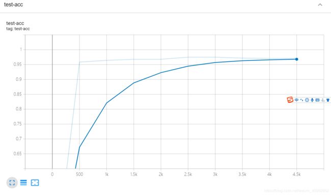
输出为：

4100 loss: 0.05817580223083496
4200 loss: 0.08532523363828659
4300 loss: 0.044528260827064514
4400 loss: 0.045207079499959946
4500 loss: 0.03408966213464737
4500 Evaluate Acc: 0.9707532051282052
4600 loss: 0.05267304927110672

运行代码后，tensorboard每过30秒更新一次。