PyTorch 01:深度学习工具 PyTorch 简介
在此 notebook 中,你将了解 PyTorch,一款用于构建和训练神经网络的框架。PyTorch 在很多方面都和 Numpy 数组很像。毕竟,这些 Numpy 数组也是张量。PyTorch 会将这些张量当做输入并使我们能够轻松地将张量移到 GPU 中,以便在训练神经网络时加快处理速度。它还提供了一个自动计算梯度的模块(用于反向传播),以及另一个专门用于构建神经网络的模块。总之,与 TensorFlow 和其他框架相比,PyTorch 与 Python 和 Numpy/Scipy 堆栈更协调。
神经网络
深度学习以人工神经网络为基础。人工神经网络大致产生于上世纪 50 年代末。神经网络由多个像神经元一样的单个部分组成,这些部分通常称为单元或直接叫做“神经元”。每个单元都具有一定数量的加权输入。我们对这些加权输入求和,然后将结果传递给激活函数,以获得单元的输出。
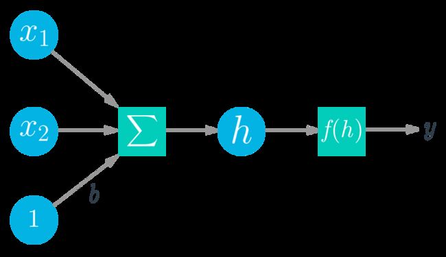
数学公式如下所示:
y = f ( w 1 x 1 + w 2 x 2 + b ) y = f(w_1 x_1 + w_2 x_2 + b) y=f(w1x1+w2x2+b)
y = f ( ∑ i w i x i + b ) y = f\left(\sum_i w_i x_i +b \right) y=f(i∑wixi+b)
对于向量来说,为两个向量的点积/内积:
h = [ x 1 x 2 ⋯ x n ] ⋅ [ w 1 w 2 ⋮ w n ] h = \begin{bmatrix} x_1 \, x_2 \cdots x_n \end{bmatrix} \cdot \begin{bmatrix} w_1 \\ w_2 \\ \vdots \\ w_n \end{bmatrix} h=[x1x2⋯xn]⋅⎣⎢⎢⎢⎡w1w2⋮wn⎦⎥⎥⎥⎤
张量
实际上神经网络计算只是对张量进行一系列线性代数运算,张量是矩阵的泛化形式。向量是一维张量,矩阵是二维张量,包含 3 个索引的数组是三维张量(例如 RGB 彩色图像)。神经网络的基本数据结构是张量,PyTorch(以及几乎所有其他深度学习框架)都是以张量为基础。

这些是基本知识,我们现在来看 PyTorch 如何构建简单的神经网络。
# First, import PyTorch
import torch
def activation(x):
    """ Sigmoid activation function

        Arguments
        ---------
        x: torch.Tensor
    """
    return 1/(1+torch.exp(-x))
### Generate some data
torch.manual_seed(7) # Set the random seed so things are predictable

# Features are 3 random normal variables
features = torch.randn((1, 5))
# True weights for our data, random normal variables again
weights = torch.randn_like(features)
# and a true bias term
bias = torch.randn((1, 1))
print(features.shape)
print(weights.shape)
torch.Size([1, 5])
torch.Size([1, 5])
我在上面生成了一些数据,我们可以使用该数据获取这个简单网络的输出。这些暂时只是随机数据,之后我们将使用正常数据。我们来看看:
features = torch.randn((1, 5)) 创建一个形状为 (1, 5) 的张量,其中有 1 行和 5 列,包含根据正态分布(均值为 0,标准偏差为 1)随机分布的值。
weights = torch.randn_like(features) 创建另一个形状和 features 一样的张量,同样包含来自正态分布的值。
最后,bias = torch.randn((1, 1)) 根据正态分布创建一个值。
和 Numpy 数组一样,PyTorch 张量可以相加、相乘、相减。行为都很类似。但是 PyTorch 张量具有一些优势,例如 GPU 加速,稍后我们会讲解。请计算这个简单单层网络的输出。
练习:计算网络的输出:输入特征为
features,权重为weights,偏差为bias。和 Numpy 类似,PyTorch 也有一个对张量求和的torch.sum()函数和.sum()方法。请使用上面定义的函数activation作为激活函数。
## Calculate the output of this network using the weights and bias tensors
y = activation(torch.sum(features*weights) + bias)
y = activation((features*weights).sum() + bias)
print(y)
tensor([[0.1595]])
你可以在同一运算里使用矩阵乘法进行乘法和加法运算。推荐使用矩阵乘法,因为在 GPU 上使用现代库和高效计算资源使矩阵乘法更高效。
如何对特征和权重进行矩阵乘法运算?我们可以使用 torch.mm() 或 torch.matmul(),后者更复杂,并支持广播。如果不对features 和 weights 进行处理,就会报错:
>> torch.mm(features, weights)

---------------------------------------------------------------------------
RuntimeError                              Traceback (most recent call last)
<ipython-input-13-15d592eb5279> in <module>()
----> 1 torch.mm(features, weights)

RuntimeError: size mismatch, m1: [1 x 5], m2: [1 x 5] at /Users/soumith/minicondabuild3/conda-bld/pytorch_1524590658547/work/aten/src/TH/generic/THTensorMath.c:2033
在任何框架中构建神经网络时,我们都会频繁遇到这种情况。原因是我们的张量不是进行矩阵乘法的正确形状。注意,对于矩阵乘法,第一个张量里的列数必须等于第二个张量里的行数。features 和 weights 具有相同的形状,即 (1, 5)。意味着我们需要更改 weights 的形状,以便进行矩阵乘法运算。
注意: 要查看张量 tensor 的形状,请使用 tensor.shape。以后也会经常用到。
现在我们有以下几个选择:weights.reshape()、weights.resize_() 和 weights.view()。
weights.reshape(a, b)有时候将返回一个新的张量,数据和weights的一样,大小为(a, b);有时候返回克隆版,将数据复制到内存的另一个部分。weights.resize_(a, b)返回形状不同的相同张量。但是,如果新形状的元素数量比原始张量的少,则会从张量里删除某些元素(但是不会从内存中删除)。如果新形状的元素比原始张量的多,则新元素在内存里未初始化。注意,方法末尾的下划线表示这个方法是原地运算。要详细了解如何在 PyTorch 中进行原地运算,请参阅此论坛话题。weights.view(a, b)将返回一个张量,数据和weights的一样,大小为(a, b)。
我通常使用 .view(),但这三个方法对此示例来说都可行。现在,我们可以通过 weights.view(5, 1) 变形 weights,使其具有 5 行和 1 列。
练习:请使用矩阵乘法计算网络的输出
## Calculate the output of this network using matrix multiplication
y = activation(torch.mm(features,weights.view(5,1)) + bias)
print(y)
tensor([[0.1595]])
堆叠
这就是计算单个神经元的输出的方式。当你将单个单元堆叠为层,并将层堆叠为神经元网络后,你就会发现这个算法的强大之处。一个神经元层的输出变成下一层的输入。对于多个输入单元和输出单元,我们现在需要将权重表示为矩阵。
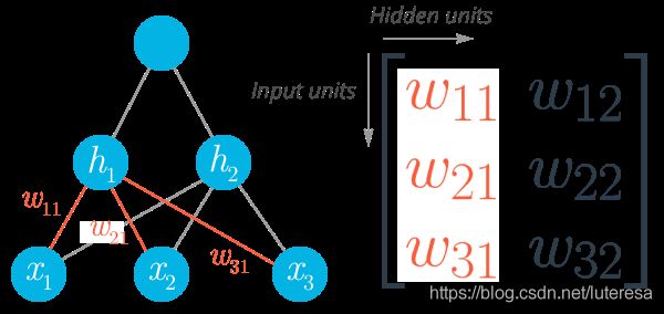
底部显示的第一个层级是输入,称为输入层。中间层称为隐藏层,最后一层(右侧)是输出层。我们可以再次使用矩阵从数学角度来描述这个网络,然后使用矩阵乘法将每个单元线性组合到一起。例如,可以这样计算隐藏层( h 1 h_1 h1 和 h 2 h_2 h2):
h ⃗ = [ h 1 h 2 ] = [ x 1 x 2 ⋯ x n ] ⋅ [ w 11 w 12 w 21 w 22 ⋮ ⋮ w n 1 w n 2 ] \vec{h} = [h_1 \, h_2] = \begin{bmatrix} x_1 \, x_2 \cdots \, x_n \end{bmatrix} \cdot \begin{bmatrix} w_{11} & w_{12} \\ w_{21} &w_{22} \\ \vdots &\vdots \\ w_{n1} &w_{n2} \end{bmatrix} h=[h1h2]=[x1x2⋯xn]⋅⎣⎢⎢⎢⎡w11w21⋮wn1w12w22⋮wn2⎦⎥⎥⎥⎤
我们可以将隐藏层当做输出单元的输入,从而得出这个小网络的输出,简单表示为:
y = f 2 ( f 1 ( x ⃗ W 1 ) W 2 ) y = f_2 \! \left(\, f_1 \! \left(\vec{x} \, \mathbf{W_1}\right) \mathbf{W_2} \right) y=f2(f1(xW1)W2)
### Generate some data
torch.manual_seed(7) # Set the random seed so things are predictable

# Features are 3 random normal variables
features = torch.randn((1, 3))
print(features.shape)

# Define the size of each layer in our network
n_input = features.shape[1]     # Number of input units, must match number of input features
n_hidden = 2                    # Number of hidden units
n_output = 1                    # Number of output units

# Weights for inputs to hidden layer
W1 = torch.randn(n_input, n_hidden)
# Weights for hidden layer to output layer
W2 = torch.randn(n_hidden, n_output)
print(W1.shape)

# and bias terms for hidden and output layers
B1 = torch.randn((1, n_hidden))
B2 = torch.randn((1, n_output))

print(B1.shape)
torch.Size([1, 3])
torch.Size([3, 2])
torch.Size([1, 2])
**练习:**使用权重
W1和W2以及偏差B1和B2计算此多层网络的输出。
## Your solution here
h = activation(torch.mm(features,W1) + B1)
output = activation(torch.mm(h,W2) + B2)
print(output)
tensor([[0.3171]])
如果计算正确,输出应该为 tensor([[ 0.3171]])。
隐藏层数量是网络的参数,通常称为超参数,以便与权重和偏差参数区分开。稍后当我们讨论如何训练网络时会提到,层级越多,网络越能够从数据中学习规律并作出准确的预测。
Numpy 和 Torch 相互转换
加分题!PyTorch 可以实现 Numpy 数组和 Torch 张量之间的转换。Numpy 数组转换为张量数据,可以用 torch.from_numpy()。张量数据转换为 Numpy 数组,可以用 .numpy() 。
import numpy as np
a = np.random.rand(4,3)
a
array([[0.85679551, 0.93626926, 0.284956  ],
       [0.18478529, 0.05775879, 0.44416887],
       [0.68360642, 0.51638607, 0.49711792],
       [0.18593368, 0.53402654, 0.23731168]])
b = torch.from_numpy(a)
b
tensor([[0.8568, 0.9363, 0.2850],
        [0.1848, 0.0578, 0.4442],
        [0.6836, 0.5164, 0.4971],
        [0.1859, 0.5340, 0.2373]], dtype=torch.float64)
b.numpy()
array([[0.85679551, 0.93626926, 0.284956  ],
       [0.18478529, 0.05775879, 0.44416887],
       [0.68360642, 0.51638607, 0.49711792],
       [0.18593368, 0.53402654, 0.23731168]])
Numpy 数组与 Torch 张量之间共享内存,因此如果你原地更改一个对象的值,另一个对象的值也会更改。
# Multiply PyTorch Tensor by 2, in place
b.mul_(2)
tensor([[1.7136, 1.8725, 0.5699],
        [0.3696, 0.1155, 0.8883],
        [1.3672, 1.0328, 0.9942],
        [0.3719, 1.0681, 0.4746]], dtype=torch.float64)
# Numpy array matches new values from Tensor
a
array([[1.71359101, 1.87253851, 0.569912  ],
       [0.36957058, 0.11551758, 0.88833775],
       [1.36721285, 1.03277214, 0.99423583],
       [0.37186737, 1.06805308, 0.47462336]])