吴恩达机器学习编程作业ex5 Regularized Linear Regression and Bias v.s. Variance

一、程序及函数

1.引导脚本ex5.m

%% Machine Learning Online Class
%  Exercise 5 | Regularized Linear Regression and Bias-Variance
%
%  Instructions
%  ------------
%  This file contains code that helps you get started on the
%  exercise. You will need to complete the following functions:
%
%     linearRegCostFunction.m
%     learningCurve.m
%     validationCurve.m
%
%  For this exercise, you will not need to change any code in this file,
%  or any other files other than those mentioned above.

%% Initialization
clear;
close all;
clc

%% =========== Part 1: Loading and Visualizing Data =============
%  We start the exercise by first loading and visualizing the dataset. 
%  The following code will load the dataset into your environment and plot the data.

% Load Training Data
fprintf('Loading and Visualizing Data ...\n')

% Load from ex5data1: 
% You will have X, y, Xval, yval, Xtest, ytest in your environment
load ('ex5data1.mat');

% m = Number of examples
m = size(X, 1);

% Plot training data
plot(X, y, 'rx', 'MarkerSize', 10, 'LineWidth', 1.5);
xlabel('Change in water level (x)');
ylabel('Water flowing out of the dam (y)');

fprintf('Program paused. Press enter to continue.\n');
pause;

%% =========== Part 2: Regularized Linear Regression Cost =============
%  You should now implement the cost function for regularized linear regression. 

theta = [1; 1];
J = linearRegCostFunction([ones(m, 1) X], y, theta, 1);

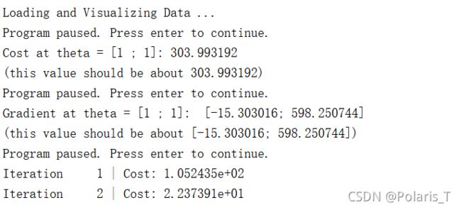
fprintf(['Cost at theta = [1 ; 1]: %f '...
         '\n(this value should be about 303.993192)\n'], J);

fprintf('Program paused. Press enter to continue.\n');
pause;

%% =========== Part 3: Regularized Linear Regression Gradient =============
%  You should now implement the gradient for regularized linear regression.

theta = [1 ; 1];
[J, grad] = linearRegCostFunction([ones(m, 1) X], y, theta, 1);

fprintf(['Gradient at theta = [1 ; 1]:  [%f; %f] '...
         '\n(this value should be about [-15.303016; 598.250744])\n'], ...
         grad(1), grad(2));

fprintf('Program paused. Press enter to continue.\n');
pause;


%% =========== Part 4: Train Linear Regression =============
%  Once you have implemented the cost and gradient correctly, the
%  trainLinearReg function will use your cost function to train 
%  regularized linear regression.
% 
%  Write Up Note: The data is non-linear, so this will not give a great 
%                 fit.
%

%  Train linear regression with lambda = 0
lambda = 0;
[theta] = trainLinearReg([ones(m, 1) X], y, lambda);

%  Plot fit over the data
plot(X, y, 'rx', 'MarkerSize', 10, 'LineWidth', 1.5);
xlabel('Change in water level (x)');
ylabel('Water flowing out of the dam (y)');
hold on;
plot(X, [ones(m, 1) X]*theta, '--', 'LineWidth', 2)
hold off;

fprintf('Program paused. Press enter to continue.\n');
pause;

%% =========== Part 5: Learning Curve for Linear Regression =============
%  Next, you should implement the learningCurve function. 
%
%  Write Up Note: Since the model is underfitting the data, we expect to
%                 see a graph with "high bias" -- Figure 3 in ex5.pdf 

lambda = 0;
[error_train, error_val] = learningCurve([ones(m, 1) X], y, ...
                           [ones(size(Xval, 1), 1) Xval], yval, lambda);

plot(1:m, error_train, 1:m, error_val);
title('Learning curve for linear regression')
legend('Train', 'Cross Validation')
xlabel('Number of training examples')
ylabel('Error')
axis([0 13 0 150])

fprintf('# Training Examples\tTrain Error\tCross Validation Error\n');
for i = 1:m
    fprintf('  \t%d\t\t%f\t%f\n', i, error_train(i), error_val(i));
end

fprintf('Program paused. Press enter to continue.\n');
pause;

%% =========== Part 6: Feature Mapping for Polynomial Regression =============
%  One solution to this is to use polynomial regression. You should now
%  complete polyFeatures to map each example into its powers

p = 8;

% Map X onto Polynomial Features and Normalize
X_poly = polyFeatures(X, p);
[X_poly, mu, sigma] = featureNormalize(X_poly);  % Normalize
% 下面的X_poly已经被标准化并且添加了第一列全1
X_poly = [ones(m, 1), X_poly];                   % Add Ones

% Map X_poly_test and normalize (using mu and sigma)
X_poly_test = polyFeatures(Xtest, p);
X_poly_test = bsxfun(@minus, X_poly_test, mu);
X_poly_test = bsxfun(@rdivide, X_poly_test, sigma);
% 下面的X_poly_test已经被标准化并且添加了第一列全1
X_poly_test = [ones(size(X_poly_test, 1), 1), X_poly_test];        % Add Ones

% Map X_poly_val and normalize (using mu and sigma)
X_poly_val = polyFeatures(Xval, p);
X_poly_val = bsxfun(@minus, X_poly_val, mu);
X_poly_val = bsxfun(@rdivide, X_poly_val, sigma);
% 下面的X_poly_val已经被标准化并且添加了第一列全1
X_poly_val = [ones(size(X_poly_val, 1), 1), X_poly_val];           % Add Ones

fprintf('Normalized Training Example 1:\n');
fprintf('  %f  \n', X_poly(1, :));

fprintf('\nProgram paused. Press enter to continue.\n');
pause;

%% =========== Part 7: Learning Curve for Polynomial Regression =============
%  Now, you will get to experiment with polynomial regression with multiple
%  values of lambda. The code below runs polynomial regression with 
%  lambda = 0. You should try running the code with different values of
%  lambda to see how the fit and learning curve change.

lambda = 0;
[theta] = trainLinearReg(X_poly, y, lambda);

% Plot training data and fit
figure(1);
plot(X, y, 'rx', 'MarkerSize', 10, 'LineWidth', 1.5);
plotFit(min(X), max(X), mu, sigma, theta, p);
xlabel('Change in water level (x)');
ylabel('Water flowing out of the dam (y)');
title (sprintf('Polynomial Regression Fit (lambda = %f)', lambda));

figure(2);
[error_train, error_val] = ...
    learningCurve(X_poly, y, X_poly_val, yval, lambda);
plot(1:m, error_train, 1:m, error_val);

title(sprintf('Polynomial Regression Learning Curve (lambda = %f)', lambda));
xlabel('Number of training examples')
ylabel('Error')
axis([0 13 0 100])
legend('Train', 'Cross Validation')

fprintf('Polynomial Regression (lambda = %f)\n\n', lambda);
fprintf('# Training Examples\tTrain Error\tCross Validation Error\n');
for i = 1:m
    fprintf('  \t%d\t\t%f\t%f\n', i, error_train(i), error_val(i));
end

fprintf('Program paused. Press enter to continue.\n');
pause;

%% =========== Part 8: Validation for Selecting Lambda =============
%  You will now implement validationCurve to test various values of 
%  lambda on a validation set. You will then use this to select the
%  "best" lambda value.

[lambda_vec, error_train, error_val] = ...
    validationCurve(X_poly, y, X_poly_val, yval);

close all;
plot(lambda_vec, error_train, lambda_vec, error_val);
legend('Train', 'Cross Validation');
xlabel('lambda');
ylabel('Error');

fprintf('lambda\t\tTrain Error\tValidation Error\n');
for i = 1:length(lambda_vec)
	fprintf(' %f\t%f\t%f\n', ...
            lambda_vec(i), error_train(i), error_val(i));
end

fprintf('Program paused. Press enter to continue.\n');
pause;

2.核心函数 linearRegCostFunction.m
该函数计算了带有正则化项的损失函数J值以及J对各个参数的偏导值。

function [J, grad] = linearRegCostFunction(X, y, theta, lambda)
%LINEARREGCOSTFUNCTION Compute cost and gradient for regularized linear 
%regression with multiple variables
%   [J, grad] = LINEARREGCOSTFUNCTION(X, y, theta, lambda) computes the 
%   cost of using theta as the parameter for linear regression to fit the 
%   data points in X and y. Returns the cost in J and the gradient in grad

% Initialize some useful values
m = length(y); % number of training examples
n = length(theta); % number of thetas
% You need to return the following variables correctly 
grad = zeros(size(theta));
% ====================== YOUR CODE HERE ======================
% Instructions: Compute the cost and gradient of regularized linear 
%               regression for a particular choice of theta.
%
%               You should set J to the cost and grad to the gradient.

% 初始化累加和
sum = 0;
sum_theta = 0;
sum_grad = zeros(n,1);
for i = 1 : m
    sum = sum + (X(i,:) * theta - y(i)).^2;
    for j = 1 : n
        sum_grad(j) = sum_grad(j) + ((X(i,:) * theta - y(i)) .* X(i,j));
    end
end

for j = 2 : n
    sum_theta = sum_theta + theta(j).^2;
end

% 计算J值
J = 1 / (2 * m) * sum + lambda / (2 * m) * sum_theta;
% 计算梯度值
grad(1) = 1 / m * sum_grad(1);
grad(2:end) = 1 / m * sum_grad(2:end) + lambda / m * theta(2:end);

% ========================================================================
grad = grad(:);

end

3.trainLinearReg.m
该函数的功能是利用Matlab自带的优化函数训练参数，最后返回最优的theta值。

function [theta] = trainLinearReg(X, y, lambda)
%TRAINLINEARREG Trains linear regression given a dataset (X, y) and a
%regularization parameter lambda
%   [theta] = TRAINLINEARREG (X, y, lambda) trains linear regression using
%   the dataset (X, y) and regularization parameter lambda. Returns the
%   trained parameters theta.
%

% Initialize Theta
initial_theta = zeros(size(X, 2), 1); 

% Create "short hand" for the cost function to be minimized
costFunction = @(t) linearRegCostFunction(X, y, t, lambda);

% Now, costFunction is a function that takes in only one argument
options = optimset('MaxIter', 200, 'GradObj', 'on');

% Minimize using fmincg
theta = fmincg(costFunction, initial_theta, options);

end

4.learningCurve.m
给出绘制训练集&交叉验证集的误差随训练集大小而改变的曲线所需要的数值。

function [error_train, error_val] = ...
    learningCurve(X, y, Xval, yval, lambda)
%LEARNINGCURVE Generates the train and cross validation set errors needed 
%to plot a learning curve
%   [error_train, error_val] = ...
%       LEARNINGCURVE(X, y, Xval, yval, lambda) returns the train and
%       cross validation set errors for a learning curve. In particular, 
%       it returns two vectors of the same length - error_train and 
%       error_val. Then, error_train(i) contains the training error for
%       i examples (and similarly for error_val(i)).
%
%   In this function, you will compute the train and test errors for
%   dataset sizes from 1 up to m. In practice, when working with larger
%   datasets, you might want to do this in larger intervals.
%

% Number of training examples
m = size(X, 1);

% You need to return these values correctly
error_train = zeros(m, 1);
error_val   = zeros(m, 1);

% ====================== YOUR CODE HERE ======================
% Instructions: Fill in this function to return training errors in 
%               error_train and the cross validation errors in error_val. 
%               i.e., error_train(i) and 
%               error_val(i) should give you the errors
%               obtained after training on i examples.
%
% Note: You should evaluate the training error on the first i training
%       examples (i.e., X(1:i, :) and y(1:i)).
%
%       For the cross-validation error, you should instead evaluate on
%       the _entire_ cross validation set (Xval and yval).
%
% Note: If you are using your cost function (linearRegCostFunction)
%       to compute the training and cross validation error, you should 
%       call the function with the lambda argument set to 0. 
%       Do note that you will still need to use lambda when running
%       the training to obtain the theta parameters.
%
% Hint: You can loop over the examples with the following:
%
%       for i = 1:m
%           % Compute train/cross validation errors using training examples 
%           % X(1:i, :) and y(1:i), storing the result in 
%           % error_train(i) and error_val(i)
%           ....
%           
%       end
%

% ---------------------- Sample Solution ----------------------

for i = 1 : m
    % 先训练得出theta向量的值
    [theta] = trainLinearReg(X(1:i, :), y(1:i), lambda);
    % 然后再计算当前训练集和整个验证集的误差
    error_train(i) = linearRegCostFunction(X(1:i, :), y(1:i), theta, 0);
    error_val(i) = linearRegCostFunction(Xval, yval, theta, 0);
    
% -------------------------------------------------------------

% =======================================================================
end

5.polyFeatures.m
为了得到更好的拟合曲线，我们需要用多项式回归（而不是简单的一次线性回归）。所以我们需要首先把特征X扩展为多维的特征矩阵。

function [X_poly] = polyFeatures(X, p)
%POLYFEATURES Maps X (1D vector) into the p-th power
%   [X_poly] = POLYFEATURES(X, p) takes a data matrix X (size m x 1) and
%   maps each example into its polynomial features where
%   X_poly(i, :) = [X(i) X(i).^2 X(i).^3 ...  X(i).^p];

% You need to return the following variables correctly.
X_poly = zeros(numel(X), p);

% ====================== YOUR CODE HERE ======================
% Instructions: Given a vector X, return a matrix X_poly where the p-th 
%               column of X contains the values of X to the p-th power.

m = length(X);
for i = 1 : m
    for j = 1 : p
        X_poly(i,j) = X(i,1).^j;
    end
end

% =========================================================================

end

6.validationCurve.m
为了绘制出训练集&交叉验证集的误差随着lambda而改变的曲线，我们首先要计算不同lambda下的两个集的误差。

function [lambda_vec, error_train, error_val] = ...
    validationCurve(X, y, Xval, yval)
%VALIDATIONCURVE Generate the train and validation errors needed to
%plot a validation curve that we can use to select lambda
%   [lambda_vec, error_train, error_val] = ...
%       VALIDATIONCURVE(X, y, Xval, yval) returns the train
%       and validation errors (in error_train, error_val)
%       for different values of lambda. You are given the training set (X,
%       y) and validation set (Xval, yval).
%

% Selected values of lambda (you should not change this)
lambda_vec = [0 0.001 0.003 0.01 0.03 0.1 0.3 1 3 10]';

% You need to return these variables correctly.
error_train = zeros(length(lambda_vec), 1);
error_val = zeros(length(lambda_vec), 1);

% ====================== YOUR CODE HERE ======================
% Instructions: Fill in this function to return training errors in 
%               error_train and the validation errors in error_val. The 
%               vector lambda_vec contains the different lambda parameters 
%               to use for each calculation of the errors, i.e, 
%               error_train(i), and error_val(i) should give 
%               you the errors obtained after training with 
%               lambda = lambda_vec(i)
%
% Note: You can loop over lambda_vec with the following:
%
%       for i = 1:length(lambda_vec)
%           lambda = lambda_vec(i);
%           % Compute train / val errors when training linear 
%           % regression with regularization parameter lambda
%           % You should store the result in error_train(i)
%           % and error_val(i)
%           ....
%           
%       end
m = size(X, 1);

for i = 1 : length(lambda_vec)
	lambda = lambda_vec(i);
    % 先训练得出theta向量的值
    % 这里的X都已经加上了第一列全1
    [theta] = trainLinearReg(X, y, lambda);
    error_train(i) = linearRegCostFunction(X, y, theta, 0);
    error_val(i) = linearRegCostFunction(Xval, yval, theta, 0);
    
% =========================================================================

end

其他函数都是Andrew Ng已经帮我们写好了的，相对不那么重要，就不贴上来了。

二、运行结果

到当训练样本数量增加时，训练误差和交叉验证误差都很高。这反映了模型中的一个高偏差问题(High Bias)——线性回归模型太简单以至于无法很好地适应训练集，即产生了欠拟合(Underfitting)的问题。


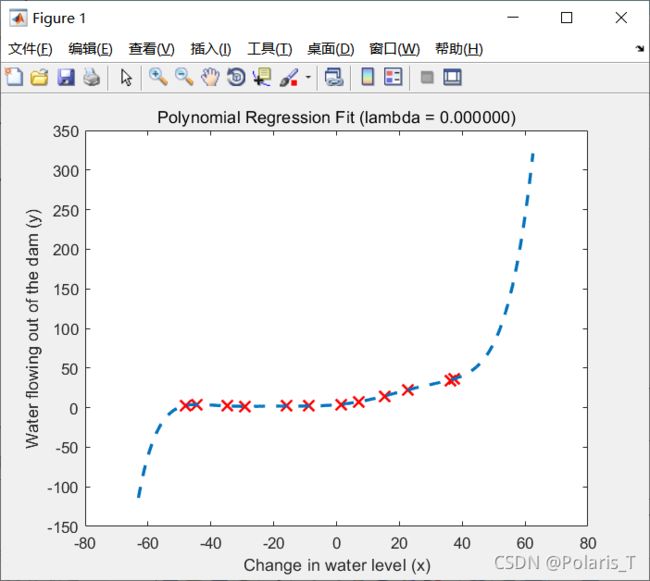
多项式回归的学习曲线：
观察曲线我们可以发现，训练误差一直很低但是交叉验证误差比训练误差要大很多，即训练误差和交叉验证误差之间存在较大差距。这表明当前的多项式回归模型存在高方差(High Variance)问题，也即模型存在过拟合(Overfitting)的问题。

一个好的lambda值要在减小J值和防止模型出现过拟合之间达到一个较好的平衡状态（这取决于实际需求）。在本问题中我们可以发现当lambda = 3时，验证集上的误差最小，说明lambda = 3是一个比较理想的值。