钉钉杯初赛A题建模-多模型融合预测银行卡诈骗模型（详细代码、解释）

钉钉杯初赛A题建模-多模型融合预测银行卡诈骗模型

前言：

8月10结束的钉钉杯a题，整体简单，建模整体代码分享如下，主要是进行了多个模型投票法融合的模型。

数据+全部代码：

链接：https://pan.baidu.com/s/1SZtLsuPHSmlaOy111uW_YA
提取码：xx78

1、对数据进行前两列特征数据进行标准化

2、采用上采样和下采样进行数据处理，使数据极不平衡得到处理

3、使用上采样和下采样的数据分别用第一阶段的5个模型进行训练和预测

4、模型优化，使用roc_auc曲线选出最好的三个模型进行保存，在第三阶段进行模型融合

5、加载四个模型融合为一个模型

6、对融合后的模型进行训练和模型评估

7、混淆矩阵查看模型的效果

数据读取与查看

读取数据

import pandas as pd
import numpy as np
df=pd.read_csv("数据集/card_transdata.csv",encoding='utf-8')  #文件路径为绝对路径，根据自己电脑文件夹的路径修改
df    

	distance_from_home	distance_from_last_transaction	ratio_to_median_purchase_price	repeat_retailer	used_chip	used_pin_number	online_order	fraud
0	57.877857	0.311140	1.945940	1.0	1.0	0.0	0.0	0.0
1	10.829943	0.175592	1.294219	1.0	0.0	0.0	0.0	0.0
2	5.091079	0.805153	0.427715	1.0	0.0	0.0	1.0	0.0
3	2.247564	5.600044	0.362663	1.0	1.0	0.0	1.0	0.0
4	44.190936	0.566486	2.222767	1.0	1.0	0.0	1.0	0.0
...	...	...	...	...	...	...	...	...
999995	2.207101	0.112651	1.626798	1.0	1.0	0.0	0.0	0.0
999996	19.872726	2.683904	2.778303	1.0	1.0	0.0	0.0	0.0
999997	2.914857	1.472687	0.218075	1.0	1.0	0.0	1.0	0.0
999998	4.258729	0.242023	0.475822	1.0	0.0	0.0	1.0	0.0
999999	58.108125	0.318110	0.386920	1.0	1.0	0.0	1.0	0.0

1000000 rows × 8 columns

查看数据情况

df.info()

RangeIndex: 1000000 entries, 0 to 999999
Data columns (total 8 columns):
 #   Column                          Non-Null Count    Dtype  
---  ------                          --------------    -----  
 0   distance_from_home              1000000 non-null  float64
 1   distance_from_last_transaction  1000000 non-null  float64
 2   ratio_to_median_purchase_price  1000000 non-null  float64
 3   repeat_retailer                 1000000 non-null  float64
 4   used_chip                       1000000 non-null  float64
 5   used_pin_number                 1000000 non-null  float64
 6   online_order                    1000000 non-null  float64
 7   fraud                           1000000 non-null  float64
dtypes: float64(8)
memory usage: 61.0 MB

• 数据的类型基本是float64。即都是数字形式
• 数据中没有空行

# 介绍数据集各列的 数据统计情况
df.describe() 

	distance_from_home	distance_from_last_transaction	ratio_to_median_purchase_price	repeat_retailer	used_chip	used_pin_number	online_order	fraud
count	1000000.000000	1000000.000000	1000000.000000	1000000.000000	1000000.000000	1000000.000000	1000000.000000	1000000.000000
mean	26.628792	5.036519	1.824182	0.881536	0.350399	0.100608	0.650552	0.087403
std	65.390784	25.843093	2.799589	0.323157	0.477095	0.300809	0.476796	0.282425
min	0.004874	0.000118	0.004399	0.000000	0.000000	0.000000	0.000000	0.000000
25%	3.878008	0.296671	0.475673	1.000000	0.000000	0.000000	0.000000	0.000000
50%	9.967760	0.998650	0.997717	1.000000	0.000000	0.000000	1.000000	0.000000
75%	25.743985	3.355748	2.096370	1.000000	1.000000	0.000000	1.000000	0.000000
max	10632.723672	11851.104565	267.802942	1.000000	1.000000	1.000000	1.000000	1.000000

• 可以观察到distance_from_home（银行卡交易地点与家的距离）和distance_from_last_transaction（与上次交易发生的距离）的方差相对于其他特征很大

数据分析可视化

print('distance_from_home不是诈骗统计：'+str(len(df.loc[(df['fraud'] == 0),'distance_from_home'])))
print('distance_from_home是诈骗统计：'+str(len(df.loc[(df['fraud'] == 1),'distance_from_home'])))

print('distance_from_last_transaction不是诈骗统计：'+str(len(df.loc[(df['fraud'] == 0),'distance_from_last_transaction'])))
print('distance_from_last_transaction是诈骗统计：'+str(len(df.loc[(df['fraud'] == 1),'distance_from_last_transaction'])))

print('ratio_to_median_purchase_price不是诈骗统计：'+str(len(df.loc[(df['fraud'] == 0),'ratio_to_median_purchase_price'])))
print('ratio_to_median_purchase_price是诈骗统计：'+str(len(df.loc[(df['fraud'] == 1),'ratio_to_median_purchase_price'])))

distance_from_home不是诈骗统计：912597
distance_from_home是诈骗统计：87403
distance_from_last_transaction不是诈骗统计：912597
distance_from_last_transaction是诈骗统计：87403
ratio_to_median_purchase_price不是诈骗统计：912597
ratio_to_median_purchase_price是诈骗统计：87403

查看正负样本数量：

from pyecharts.charts import Pie
from pyecharts import options as opts
L1=['fraud','Not fraud']
num=[87403,912597]
c=Pie()
c.add("",[list(z) for z in zip(L1,num)])
c.set_global_opts(title_opts=opts.TitleOpts(title="正负样本分布")) 
c.set_series_opts(label_opts=opts.LabelOpts(formatter="{b}:{c}"))
c.render_notebook()

     

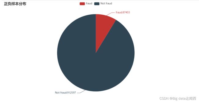
• 从中我们可以观察到，正样本数量远远大于负样本数量，正负样本数量不均衡。

• 大部分分类器的输出类别是基于阈值的，如小于0.5的为反例，大于则为正例。在数据不平衡时，默认的阈值会导致模型输出倾向与类别数据多的类别

• 这里我们采用下采样的方法平衡数据

  下采样 ：从大量的正样本中挑选若干个，使得正样本和负样本数目一样小

观察distance_from_home和是否诈骗的关系

#### 观察distance和是否诈骗的关系
import matplotlib.pyplot as plt

# 构建两个子图
f, (ax1, ax2) = plt.subplots(2, 1, sharex=True, figsize=(16,4))

# 设置柱状宽度
bins = 30

# 统计欺诈案例的交易金额
ax1.hist(df["distance_from_home"][df["fraud"]== 1], bins = bins)
ax1.set_title('Fraud')

# 统计正常案例的交易金额
ax2.hist(df["distance_from_home"][df["fraud"] == 0], bins = bins)
ax2.set_title('Not Fraud')

# 画坐标系
plt.xlabel('distance')
plt.ylabel('Number of Transactions')
plt.yscale('log')

plt.show()    # 展示图像

​

​

• k可以看出咋骗集中在distance大约为500以内，说明可能是同城诈骗居多。

观察distance_from_last_transaction：和是否诈骗的关系

#### 观察distance和是否诈骗的关系
import matplotlib.pyplot as plt

# 构建两个子图
f, (ax1, ax2) = plt.subplots(2, 1, sharex=True, figsize=(16,4))

# 设置柱状宽度
bins = 30

# 统计欺诈案例的交易金额
ax1.hist(df["distance_from_last_transaction"][df["fraud"]== 1], bins = bins)
ax1.set_title('Fraud')

# 统计正常案例的交易金额
ax2.hist(df["distance_from_last_transaction"][df["fraud"] == 0], bins = bins)
ax2.set_title('Not Fraud')

# 画坐标系
plt.xlabel('distance')
plt.ylabel('Number of Transactions')
plt.yscale('log')

plt.show()    # 展示图像

​

​

同城诈骗，可能距离小不容易引起怀疑

观察各个特征之间的联系

import seaborn as sns

# 创建图像
grid_kws = {"width_ratios": (.9, .9, .05), "wspace": 0.2}
f, (ax1, ax2, cbar_ax) = plt.subplots(1, 3, gridspec_kw=grid_kws, figsize = (18, 9))

# 定义调色板
cmap = sns.diverging_palette(220, 8, as_cmap=True)

# 计算正常案例中的特征联系
correlation_NonFraud = df[df["fraud"] == 0].loc[:, df.columns != 'fraud'].corr()
# 计算欺诈案例中的特征联系
correlation_Fraud = df[df["fraud"] == 1].loc[:, df.columns != 'fraud'].corr()
# 计算上三角mask矩阵
mask = np.zeros_like(correlation_NonFraud)
indices = np.triu_indices_from(correlation_NonFraud)
mask[indices] = True


# 画正常案例的特征联系热力图
ax1 =sns.heatmap(correlation_NonFraud, ax = ax1, vmin = -1, vmax = 1, cmap = cmap, square = False, \
                 linewidths = 0.5, mask = mask, cbar = False)
ax1.set_xticklabels(ax1.get_xticklabels(), size = 16); 
ax1.set_yticklabels(ax1.get_yticklabels(), size = 16); 
ax1.set_title('Normal', size = 20)

# 画欺诈案例的特征联系热力图
ax2 = sns.heatmap(correlation_Fraud, vmin = -1, vmax = 1, cmap = cmap, ax = ax2, square = False, \
                  linewidths = 0.5, mask = mask, yticklabels = False, \
                  cbar_ax = cbar_ax, cbar_kws={'orientation': 'vertical',  'ticks': [-1, -0.5, 0, 0.5, 1]})

ax2.set_xticklabels(ax2.get_xticklabels(), size = 16); 
ax2.set_title('Fraud', size = 20);

cbar_ax.set_yticklabels(cbar_ax.get_yticklabels(), size = 14);

plt.show()    # 展示图像

​

​

df.corr()

	distance_from_home	distance_from_last_transaction	ratio_to_median_purchase_price	repeat_retailer	used_chip	used_pin_number	online_order	fraud
distance_from_home	1.000000	0.000193	-0.001374	0.143124	-0.000697	-0.001622	-0.001301	0.187571
distance_from_last_transaction	0.000193	1.000000	0.001013	-0.000928	0.002055	-0.000899	0.000141	0.091917
ratio_to_median_purchase_price	-0.001374	0.001013	1.000000	0.001374	0.000587	0.000942	-0.000330	0.462305
repeat_retailer	0.143124	-0.000928	0.001374	1.000000	-0.001345	-0.000417	-0.000532	-0.001357
used_chip	-0.000697	0.002055	0.000587	-0.001345	1.000000	-0.001393	-0.000219	-0.060975
used_pin_number	-0.001622	-0.000899	0.000942	-0.000417	-0.001393	1.000000	-0.000291	-0.100293
online_order	-0.001301	0.000141	-0.000330	-0.000532	-0.000219	-0.000291	1.000000	0.191973
fraud	0.187571	0.091917	0.462305	-0.001357	-0.060975	-0.100293	0.191973	1.000000

从上图可以看出

• 在银行卡诈骗事件中，变量distance_from_home、ratio_to_median_purchase_price、repeat_retailer与属于诈骗有较强的

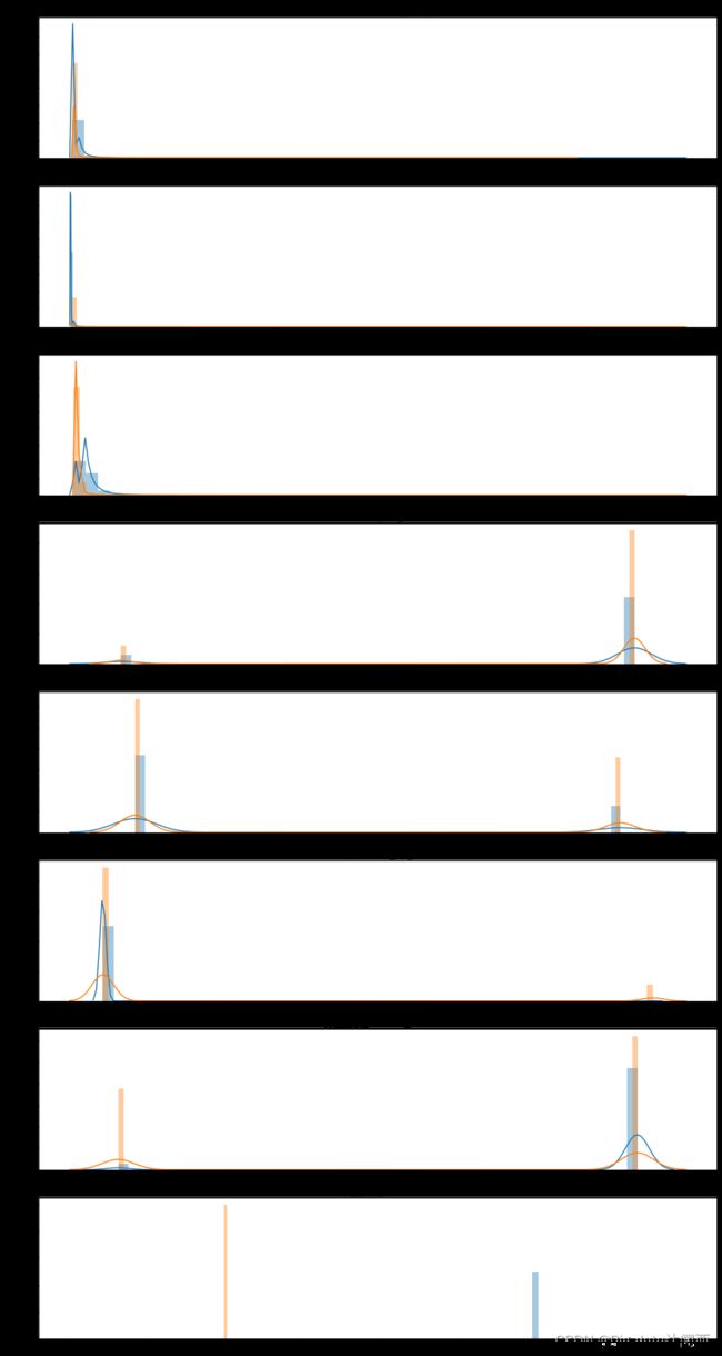
观察各个特征分布

import matplotlib.pyplot as plt
import matplotlib.gridspec as gridspec
import seaborn as sns
# 特征名
feature_num = len(df.columns)
v_feat = list(df.columns)

# 构建图像
plt.figure(figsize=(16,feature_num*4))
gs = gridspec.GridSpec(feature_num, 1) 

for i, cn in enumerate(df[v_feat]):
    ax = plt.subplot(gs[i])
    sns.distplot(df[cn][df["fraud"] == 1], bins=50)
    sns.distplot(df[cn][df["fraud"] == 0], bins=100)
    ax.set_xlabel('')
    ax.set_title('特征直方图: ' + str(cn))
plt.rcParams['font.sans-serif']=['SimHei']
plt.show()    # 展示图像

​

特征工程

数据标准化

# 统一导入工具包
import numpy as np
import pandas as pd
import os

from sklearn.preprocessing import StandardScaler
from sklearn.compose import ColumnTransformer
from sklearn.model_selection import train_test_split, GridSearchCV
from sklearn.ensemble import RandomForestClassifier
from sklearn.metrics import roc_auc_score, classification_report, roc_curve, auc, plot_confusion_matrix, precision_score, recall_score, f1_score 

from imblearn.over_sampling import SMOTE
from imblearn.under_sampling import RandomUnderSampler
from imblearn.pipeline import Pipeline
from joblib import dump, load

import matplotlib.pyplot as plt
import matplotlib.gridspec as gridspec
import seaborn as sns

# 观察特征返回每列的标准偏差
df.var()  

distance_from_home                4275.954684
distance_from_last_transaction     667.865469
ratio_to_median_purchase_price       7.837698
repeat_retailer                      0.104430
used_chip                            0.227620
used_pin_number                      0.090486
online_order                         0.227334
fraud                                0.079764
dtype: float64

• 前两个方差太大，我们需要对其进行标准化 因为模型会对方差较大的特征值误认为它对与分类有着较大的权重，因此把数据大小劲量均衡

### 单独使用StandardScaler()进行标准化
from sklearn.preprocessing import StandardScaler
old_dfh = df['distance_from_home'].values.reshape(-1, 1)
# print(old_amount)
print('distance_from_home标准化之前的方差', old_dfh.std())

norm_dfh = StandardScaler().fit_transform(df['distance_from_home'].values.reshape(-1, 1))

print('distance_from_home标准化之后的方差', norm_dfh.std())

### 单独使用StandardScaler()进行标准化
from sklearn.preprocessing import StandardScaler
old_dflt = df['distance_from_last_transaction'].values.reshape(-1, 1)
# print(old_amount)
print('distance_from_last_transaction标准化之前的方差', old_dflt.std())

norm_dflt = StandardScaler().fit_transform(df['distance_from_last_transaction'].values.reshape(-1, 1))

print('distance_from_last_transaction标准化之后的方差', norm_dflt.std())

distance_from_home标准化之前的方差 65.39075170364431
distance_from_home标准化之后的方差 1.0000000000000004
distance_from_last_transaction标准化之前的方差 25.843080339696936
distance_from_last_transaction标准化之后的方差 1.0

# 封装到ColumnTransformer中，方便后续调用标准化操作
column_trans = Pipeline([('scaler', StandardScaler())])

preprocessing = ColumnTransformer(
    transformers=[
        ('column_trans', column_trans, ['distance_from_home','distance_from_last_transaction'])
    ], remainder='passthrough'
)

过采样与欠采样数据处理

• SMOTE算法过采样的思想是合成新的少数类样本，合成的策略是对每个少数类样本a，从它的最近邻中随机选一个样本b，然后在a、b之间的连线上随机选一点作为新合成的少数类样本。

• 如果采用欠采样的方法，通常是对数目较多的那一类样本进行随机挑选样本，使得两类样本数目相等。这种做法会抛弃了大部分数据。

划分数据集

x = df.drop('fraud',axis=1)
x
y = df['fraud']
y

X_train, X_test, y_train, y_test = train_test_split(x, y, test_size=0.2, random_state=42) 

#查看维度
print('x_train.shape:',X_train.shape)
print('y_train.shape:',y_train.shape)
print('x_test.shape:',X_test.shape)
print('y_test.shape:',y_test.shape)

x_train.shape: (800000, 7)
y_train.shape: (800000,)
x_test.shape: (200000, 7)
y_test.shape: (200000,)

SMOTE过采样

### 单独使用SMOTE的结果
# 利用SMOTE进行过采样

print('过采样前，1的样本的个数为：',len(y_train[y_train==1]))
print('过采样前，0的样本的个数为：',len(y_train[y_train==0]))
over_sampler=SMOTE(random_state=0)
X_os_train,y_os_train=over_sampler.fit_resample(X_train,y_train)
print('过采样后，1的样本的个数为：',len(y_os_train[y_os_train==1]))
print('过采样后，0的样本的个数为：',len(y_os_train[y_os_train==0]))

过采样前，1的样本的个数为： 69960
过采样前，0的样本的个数为： 730040
过采样后，1的样本的个数为： 730040
过采样后，0的样本的个数为： 730040

随机欠采样

### 单独使用随机欠采样的结果

print('欠采样前，1的样本的个数为：',len(y_train[y_train==1]))
print('欠采样前，0的样本的个数为：',len(y_train[y_train==0]))
under_sampler=RandomUnderSampler(random_state=0) 
X_us_train,y_us_train=under_sampler.fit_resample(X_train,y_train)
print('欠采样后，1的样本的个数为：',len(y_us_train[y_us_train==1]))
print('欠采样后，0的样本的个数为：',len(y_us_train[y_us_train==0]))

欠采样前，1的样本的个数为： 69960
欠采样前，0的样本的个数为： 730040
欠采样后，1的样本的个数为： 69960
欠采样后，0的样本的个数为： 69960

流水线建构模型

数据在进行模型拟合之前，需要先将数据进行输入标准化等操作转换为新数据，对于新数据，模型的预测和评估都需要进行多次转换。使用Pipeline（流水线）技术可以将数据处理和模型拟合结合在一起，减少代码量。

Pipeline 的中间过程由sklearn相适配的转换器（transformer）构成，最后一步是一个estimator（模型）。中间的节点都可以执行fit和transform方法，这样预处理都可以封装进去；最后节点只需要实现fit方法

from sklearn.linear_model import SGDClassifier      # 随机梯度
from sklearn.neighbors import KNeighborsClassifier  # K近邻
from sklearn.tree import DecisionTreeClassifier     # 决策树
from sklearn.ensemble import RandomForestClassifier # 随机森林
from sklearn.model_selection import cross_val_score # 交叉验证计算accuracy
from sklearn.model_selection import GridSearchCV    # 网格搜索，获取最优参数
from sklearn.model_selection import StratifiedKFold # 交叉验证
from collections import Counter
from xgboost import XGBClassifier
# 评估指标
from sklearn.metrics import confusion_matrix, precision_score, recall_score, f1_score, roc_auc_score, accuracy_score, classification_report

from sklearn.ensemble import BaggingClassifier # 集成学习
   

过采样流水线模型训练分数

classifiers = {
    "KNN":KNeighborsClassifier(),              # K近邻
    'DT':DecisionTreeClassifier(),             # 决策树
    'RFC':RandomForestClassifier(),            # 随机森林
    'Bagging':BaggingClassifier(),             # 集成学习bagging
    'SGD':SGDClassifier(),                      #随机梯度
    'XGB':XGBClassifier()                       #XGBoost算法
   
}

def accuracy_scores(x_train, y_train):
    for key, classifier in classifiers.items(): # 遍历每一个分类器，分别训练、计算得分
        over_pipe = Pipeline([
        ('preprocessing', preprocessing),
        ('sampler', SMOTE() ), # 数据高度不平衡，因此使用SMOTE对少数类进行过采样
        ('classifier',classifier)
        ])
        over_pipe.fit(x_train, y_train)
        training_score = cross_val_score(over_pipe, x_train, y_train, cv=5) # 5折交叉验证
        print("Classifier Name : ", classifier.__class__.__name__,"  Training Score ：", round(training_score.mean(), 4)*100,'%')

print("过采样的各个分类模型的训练分数：")
accuracy_scores(X_train,y_train)

过采样的各个分类模型的训练分数：
Classifier Name :  KNeighborsClassifier   Training Score ： 99.8 %
Classifier Name :  DecisionTreeClassifier   Training Score ： 100.0 %
Classifier Name :  RandomForestClassifier   Training Score ： 100.0 %
Classifier Name :  BaggingClassifier   Training Score ： 100.0 %
Classifier Name :  SGDClassifier   Training Score ： 92.77 %
Classifier Name :  XGBClassifier   Training Score ： 100.0 %

欠采样流水线模型训练分数

def under_accuracy_scores(x_train, y_train):
    for key, classifier in classifiers.items(): # 遍历每一个分类器，分别训练、计算得分
        # 欠采样
        under_pipe = Pipeline([
            ('preprocessing', preprocessing),
            ('sampler', RandomUnderSampler() ), # The data is highly imbalanced, hence undersample majority class with RandomUnderSampler 
            ('classifier', classifier)
        ])
        under_pipe.fit(x_train, y_train)
        training_score = cross_val_score(under_pipe, x_train, y_train, cv=5) # 5折交叉验证
        print("Classifier Name : ", classifier.__class__.__name__,"  Training Score ：", round(training_score.mean(), 4)*100,'%')

print("欠采样的各个分类模型的训练分数：")
under_accuracy_scores(X_train,y_train)

欠采样的各个分类模型的训练分数：
Classifier Name :  KNeighborsClassifier   Training Score ： 99.26 %
Classifier Name :  DecisionTreeClassifier   Training Score ： 99.99 %
Classifier Name :  RandomForestClassifier   Training Score ： 99.99 %
Classifier Name :  BaggingClassifier   Training Score ： 99.99 %
Classifier Name :  SGDClassifier   Training Score ： 92.46 %
Classifier Name :  XGBClassifier   Training Score ： 99.99 %

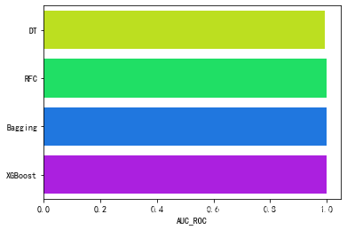
综上过采样和欠采样的模型训练分数：

• 过采样的模型比欠采样的模型训练分数高

• 在过采样模型中 ，决策树模型、随机森林模型、Bagging模型、XGBoost模型的训练分数达到了100%，我们选择这四个模型作为分类模型，

• 后面对这四个模型进行最优参数搜索、融合模型

网格搜索，得到每个模型的最优参数模型

• cross_val_score ：

一般用于获取每折的交叉验证的得分，然后根据这个得分为模型选择合适的超参数，通常需要编写循环手动完成交叉验证过程；

• GridSearchCV ：

除了自行完成叉验证外，还返回了最优的超参数及对应的最优模型
所以相对于cross_val_score来说，GridSearchCV在使用上更为方便；但是对于细节理解上，手动实现循环调用cross_val_score会更好些。

#1、决策树模型最优参数寻找
def DT_gs(x_train, y_train):
    DT_param = {
        'classifier__criterion':['gini', 'entropy'],          # 衡量标准
        'classifier__max_depth':list(range(2, 5, 1)),         # 树的深度
        'classifier__min_samples_leaf':list(range(2, 7, 1))   # 最小叶子节点数
        
        
    } 
    DT_pipe =Pipeline([ 
        ('preprocessing', preprocessing),
        ('sampler', SMOTE() ), # 数据高度不平衡，因此使用SMOTE对少数类进行过采样
        ('classifier',DecisionTreeClassifier())
        ]) 
    dt_gs = GridSearchCV(estimator=DT_pipe,param_grid=DT_param, n_jobs=-1,verbose=50, cv=4, scoring='roc_auc')
    dt_gs.fit(x_train, y_train)

    dt_best_estimators = dt_gs.best_estimator_ # 最优参数
    
    return dt_best_estimators

# 2、随机森林最优参数选择
def RFC_gs(x_train, y_train):
    grid_search_models = {
        'classifier__n_estimators': [25,50,75,100,200] # 仅作示例，可以选择其他参数
    }
    RFC_over_pipe = Pipeline([
            ('preprocessing', preprocessing),
            ('sampler', SMOTE() ), # 数据高度不平衡，因此使用SMOTE对少数类进行过采样
            ('classifier',RandomForestClassifier())
            ])
    pipe = GridSearchCV(RFC_over_pipe, grid_search_models, verbose=50, cv=5, scoring='roc_auc')
    pipe.fit(x_train, y_train)
    bst = pipe.best_estimator_ # 最优参数
    return bst

   

# 3、Bagging模型最优参数选择
def bag_gs(x_train, y_train):
    BAG_param = {
        'classifier__n_estimators':[10, 15, 20]      #集成的基估计器的个数
    }
    bag_over_pipe = Pipeline([
            ('preprocessing', preprocessing),
            ('sampler', SMOTE() ), # 数据高度不平衡，因此使用SMOTE对少数类进行过采样
            ('classifier',BaggingClassifier())
            ])
    bag_over_pipe = GridSearchCV(bag_over_pipe, BAG_param, verbose=50, cv=5, scoring='roc_auc')
    bag_over_pipe.fit(x_train, y_train)
    bag_bst = bag_over_pipe.best_estimator_ # 最优参数
    return bag_bst

# 3、XGBoost模型最优参数选择

def xgb_gs(x_train, y_train):
    XGB_param = {
        'classifier__max_depth':[3,4,5,6]
    }
    xgb_over_pipe = Pipeline([
            ('preprocessing', preprocessing),
            ('sampler', SMOTE() ), # 数据高度不平衡，因此使用SMOTE对少数类进行过采样
            ('classifier',XGBClassifier()) 
            ])
    xgb_over_pipe = GridSearchCV(xgb_over_pipe, XGB_param, verbose=50, cv=5, scoring='roc_auc')
    xgb_over_pipe.fit(x_train, y_train)
    xgb_bst = xgb_over_pipe.best_estimator_ # 最优参数
    return xgb_bst

#  得到最优参数模型
DT_best_estimator = DT_gs(X_train, y_train)

RFC_best_estimator = RFC_gs(X_train, y_train)

BAG_best_estimator = bag_gs(X_train, y_train)

XGB_best_estimator = xgb_gs(X_train,y_train)

print('4个模型最优参数：')

print('DT_best_estimator:',DT_best_estimator)
print('RFC_best_estimator:',RFC_best_estimator)
print('BAG_best_estimator:',BAG_best_estimator)
print('XGB_best_estimator:',XGB_best_estimator)

4个模型最优参数：
DT_best_estimator: Pipeline(steps=[('preprocessing',
                 ColumnTransformer(remainder='passthrough',
                                   transformers=[('column_trans',
                                                  Pipeline(steps=[('scaler',
                                                                   StandardScaler())]),
                                                  ['distance_from_home',
                                                   'distance_from_last_transaction'])])),
                ('sampler', SMOTE()),
                ('classifier',
                 DecisionTreeClassifier(max_depth=4, min_samples_leaf=4))])
RFC_best_estimator: Pipeline(steps=[('preprocessing',
                 ColumnTransformer(remainder='passthrough',
                                   transformers=[('column_trans',
                                                  Pipeline(steps=[('scaler',
                                                                   StandardScaler())]),
                                                  ['distance_from_home',
                                                   'distance_from_last_transaction'])])),
                ('sampler', SMOTE()),
                ('classifier', RandomForestClassifier(n_estimators=75))])
BAG_best_estimator: Pipeline(steps=[('preprocessing',
                 ColumnTransformer(remainder='passthrough',
                                   transformers=[('column_trans',
                                                  Pipeline(steps=[('scaler',
                                                                   StandardScaler())]),
                                                  ['distance_from_home',
                                                   'distance_from_last_transaction'])])),
                ('sampler', SMOTE()), ('classifier', BaggingClassifier())])
XGB_best_estimator: Pipeline(steps=[('preprocessing',
                 ColumnTransformer(remainder='passthrough',
                                   transformers=[('column_trans',
                                                  Pipeline(steps=[('scaler',
                                                                   StandardScaler())]),
                                                  ['distance_from_home',
                                                   'distance_from_last_transaction'])])),
                ('sampler', SMOTE()),
                ('classifier',
                 XGBClassifier(base_score=0.5, booster='gbtree', callbacks=None,
                               colsample_bylevel=1, colsample_bynode=1,
                               colsa...
                               gamma=0, gpu_id=-1, grow_policy='depthwise',
                               importance_type=None, interaction_constraints='',
                               learning_rate=0.300000012, max_bin=256,
                               max_cat_to_onehot=4, max_delta_step=0,
                               max_depth=3, max_leaves=0, min_child_weight=1,
                               missing=nan, monotone_constraints='()',
                               n_estimators=100, n_jobs=0, num_parallel_tree=1,
                               predictor='auto', random_state=0, reg_alpha=0,
                               reg_lambda=1, ...))])

保存最优参数的四个模型

import joblib as jl
#保存决策树模型：
jl.dump(DT_best_estimator,'./模型保存/dt.pkl')
#保存随机森林模型：
jl.dump(RFC_best_estimator,'./模型保存/rfc.pkl')
#保存bagging模型：
jl.dump(BAG_best_estimator,'./模型保存/bag.pkl')
#保存xgboost模型：
jl.dump(XGB_best_estimator,'./模型保存/xgb.pkl')

四个模型模型评估

评估指标数据

用 precision_recall_fscore_support 可以同时计算真实值和预测值之间的精确率、召回率、F 值、支持度。支持度为在真实值每一类出现的事件次数。

from sklearn.metrics import precision_recall_fscore_support
from sklearn.metrics import accuracy_score



def caculate(models, x_test, y_test):
    # 计算各种参数的值
    accuracy_results = []
    F1_score_results = []
    Recall_results = []
    Precision_results = []
    AUC_ROC_results = []
    
    for model in models:
        y_pred = model.predict(x_test)
        accuracy = accuracy_score(y_test, y_pred) # 计算准确度
        precision, recall, f1_score, _ = precision_recall_fscore_support(y_test, y_pred) # 计算：精确度，召回率，f1_score
        AUC_ROC = roc_auc_score(y_test, y_pred) # 计算AUC
        
        # 保存计算值
        accuracy_results.append(round(accuracy,4))
        F1_score_results.append(round(f1_score.mean(),4))
        Recall_results.append(round(recall.mean(),4))
        AUC_ROC_results.append(AUC_ROC)
        Precision_results.append(round(precision.mean(),4))
        
    return accuracy_results, F1_score_results, Recall_results, AUC_ROC_results, Precision_results

# 将所有最优超参数的模型放在一起
best_models = [ DT_best_estimator, RFC_best_estimator, BAG_best_estimator, XGB_best_estimator]

# 调用函数计算各项指标值
accuracy_results, F1_score_results, Recall_results, AUC_ROC_results, Precision_results = caculate(best_models, X_test, y_test)

# 将各项值放入到DataFrame中
result_df = pd.DataFrame(columns=['Accuracy', 'F1-score', 'Recall', 'Precision', 'AUC_ROC'],
                         index=['DT','RFC','Bagging','XGBoost'])
result_df['Accuracy'] = accuracy_results
result_df['F1-score'] = F1_score_results
result_df['Recall'] = Recall_results
result_df['Precision'] = Precision_results
result_df['AUC_ROC'] = AUC_ROC_results

result_df

	Accuracy	F1-score	Recall	Precision	AUC_ROC
DT	0.9934	0.9799	0.9927	0.9680	0.992728
RFC	1.0000	1.0000	0.9999	1.0000	0.999940
Bagging	1.0000	0.9999	0.9999	0.9999	0.999929
XGBoost	1.0000	0.9999	1.0000	0.9999	0.999986

可视化 AUC_ROC的评分.

# 可视化 AUC的评分.
g = sns.barplot('AUC_ROC', result_df.index, data=result_df, palette='hsv', orient='h')

计算各个模型的AUC值

from sklearn.model_selection import cross_val_predict
DT_pred = DT_best_estimator.predict(X_test)
RFC_pred = RFC_best_estimator.predict(X_test)
BAG_pred = BAG_best_estimator.predict(X_test)
XGB_pred = XGB_best_estimator.predict(X_test)
print(DT_pred)
print(RFC_pred)
print(BAG_pred)
print(XGB_pred)

[0. 0. 0. ... 1. 0. 0.]
[0. 0. 0. ... 1. 0. 0.]
[0. 0. 0. ... 1. 0. 0.]
[0 0 0 ... 1 0 0]

# 计算auc的评分


print('决策树模型auc分数 :', round(roc_auc_score(y_test, DT_pred),2))
print('随机森林模型auc分数 :', round(roc_auc_score(y_test, RFC_pred),2))
print('bagging模型auc分数 :', round(roc_auc_score(y_test, BAG_pred),2))
print('xgboost模型auc分数 :', round(roc_auc_score(y_test, XGB_pred),2))

决策树模型auc分数 : 0.99
随机森林模型auc分数 : 1.0
bagging模型auc分数 : 1.0
xgboost模型auc分数 : 1.0

绘制各个模型的roc曲线：

DT_fpr, DT_tpr, DT_threshold = roc_curve(y_test, DT_pred)



RFC_fpr, RFC_tpr, RFC_threshold = roc_curve(y_test, RFC_pred)

BAG_fpr, BAG_tpr, BAG_threshold = roc_curve(y_test, BAG_pred)

XGB_fpr, XGB_tpr, XGB_threshold = roc_curve(y_test, XGB_pred)

# 绘制roc曲线
def graph_roc(fpr, tpr, name, score):
    plt.figure(figsize=(8,4)) # 画布大小
    plt.title("ROC Curve", fontsize=14)
    plt.plot(fpr, tpr, 'b',label=name+"  AUC: "+ str(round(score,2)))
    plt.plot([0, 1], [0, 1], color='r', linestyle='--')
    plt.axis([-0.01, 1, 0, 1]) # 坐标轴
    plt.xlabel("False Positive Rate (FPR)", fontsize=14)
    plt.ylabel("True Positive Rate (TPR)", fontsize=14)
    plt.legend()
    plt.show()

#决策树
graph_roc(DT_fpr, DT_tpr, 'DT', roc_auc_score(y_test, DT_pred))
# 随机森林

graph_roc(RFC_fpr, RFC_tpr, 'RFC', roc_auc_score(y_test, RFC_pred))
#bag
graph_roc(BAG_fpr,BAG_tpr, 'BAG', roc_auc_score(y_test, BAG_pred))
#XGB
graph_roc(XGB_fpr,XGB_tpr, 'XGB', roc_auc_score(y_test, XGB_pred))

​

​

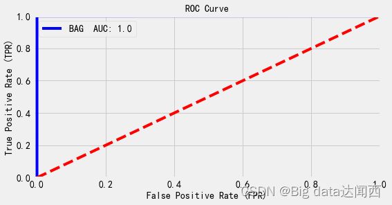
模型评估总结

，四个效果好的模型在模型评估上展现
准确率、精确率、召回率、F1值、ROC曲线、AUC 都显示很高， 说明四个模型在分类上效果显著，可信度高

加载模型、融合

import joblib 
model1 = joblib.load(filename="./模型保存/dt.pkl")
model1
model2 = joblib.load('./模型保存/rfc.pkl')
model3 = joblib.load('./模型保存/bag.pkl')
model4 = joblib.load('./模型保存/xgb.pkl')

# 将4个较好的模型集成起来，当做一个模型
from sklearn.ensemble import VotingClassifier

voting_clf = VotingClassifier(estimators=[('DT', model1), ('RFC', model2), ('BAG',model3),
                                          ('XGB', model4)], n_jobs=-1,voting='soft')
voting_clf

模型训练

import pandas as pd
import numpy as np
df=pd.read_csv("数据集/card_transdata.csv",encoding='utf-8')  #文件路径为绝对路径，根据自己电脑文件夹的路径修改
df   

x = df.drop('fraud',axis=1)
x
y = df['fraud']
y
from sklearn.model_selection import train_test_split, GridSearchCV
X_train, X_test, y_train, y_test = train_test_split(x, y, test_size=0.2, random_state=42) 

#查看维度
print('x_train.shape:',X_train.shape)
print('y_train.shape:',y_train.shape)
print('x_test.shape:',X_test.shape)
print('y_test.shape:',y_test.shape)

x_train.shape: (800000, 7)
y_train.shape: (800000,)
x_test.shape: (200000, 7)
y_test.shape: (200000,)

# 训练
voting_clf.fit(X_train, y_train)

#训练分数
from sklearn.model_selection import cross_val_score # 交叉验证计算accuracy
training_score = cross_val_score(voting_clf, X_train, y_train, cv=5) # 5折交叉验证
print("融合后模型训练分数：", round(training_score.mean(), 4)*100,'%')

融合后模型训练分数： 100.0 %

# 预测
y_final_pred = voting_clf.predict(X_test)
y_final_pred

array([0., 0., 0., ..., 1., 0., 0.])

模型评估

from sklearn.metrics import roc_auc_score, classification_report, roc_curve, auc, plot_confusion_matrix, precision_score, recall_score, f1_score 

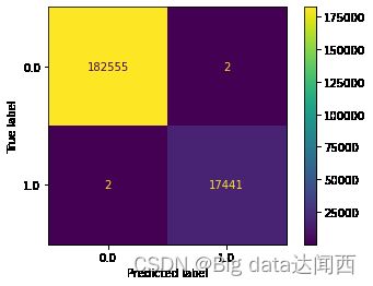
混淆矩阵

#
import matplotlib.pyplot as plt
plot_confusion_matrix(voting_clf, X_test, y_test)
plt.show()    # 展示图像

计算精确率、召回率以及综合两者的F1值

y_preds = voting_clf.predict(X_test)
p = precision_score(y_test, y_preds)
r = recall_score(y_test, y_preds)
f1 = f1_score(y_test, y_preds)

print("precision（准确率）: ", p)
print("recall（召回率）: ", r)
print("F1: ", f1)

precision（准确率）:  0.9998853408243995
recall（召回率）:  0.9998853408243995
F1:  0.9998853408243995

print(classification_report(y_test, y_preds)) #评价指标

              precision    recall  f1-score   support

         0.0       1.00      1.00      1.00    182557
         1.0       1.00      1.00      1.00     17443

    accuracy                           1.00    200000
   macro avg       1.00      1.00      1.00    200000
weighted avg       1.00      1.00      1.00    200000

​

保存融合后的模型

joblib.dump(voting_clf,'./模型保存/best_model.pkl')

最后：

创作不易，如果觉得有参考价值，请点个关注再走呗，请点个关注再走呗，请点个关注再走呗，蟹蟹