Matplotlib 和 Seaborn（Figures、Axes 和 Subplot）

Figures、Axes 和 Subplot

到目前为止，你已经见过并使用 matplotlib 和 seaborn 练习过一些基本绘制函数。上个页面介绍了新的知识：通过 matplotlib 的 subplot() 函数创建两个并排显示的图表。如果你对该函数或 figure() 函数的原理有任何疑问，请继续阅读。此页面将使用 matplotlib 讨论可视化的基本结构，以及子图表在该结构下的工作原理。

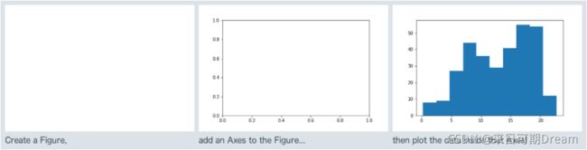
matplotlib 中的可视化基本结构是 Figure 对象。每个 Figure 中将包含一个或多个 Axes 对象，每个 Axes 对象包含多个表示每个图表的其他元素。在最早的示例中，我们隐式地创建了这些对象。假设我们在 Jupyter notebook 中运行了以下表达式，从而创建一个直方图：

plt.hist(data = df, x = 'num_var')

由于没有要在其中绘制图表的 Figure 区域，所以 Python 首先创建一个 Figure 对象。因为 Figure 没有以任何 Axes 开始来绘制直方图，所以在 Figure 里创建了一个 Axes 对象。最后，在该 Axes 中绘制直方图。

有必要了解这种对象层次结构，这样才能够更好地控制图表的布局和外观。对于上面的直方图，还有一种替代创建方式，即如下所示地显式设置 Figure 和 Axes：

fig = plt.figure()
ax = fig.add_axes([.125, .125, .775, .755])
ax.hist(data = df, x = 'num_var')

figure() 会创建一个新的 Figure 对象，我们将对它的引用存储在了变量 fig 中。其中一个 Figure 方法是 .add_axes()，它会在 Figure 中创建新的 Axes 对象。该方法需要一个列表参数，用于指定 Axes 的维度：列表中的前两个元素表示 Axes 的左下角位置（即 Figure 的左下角象限），后两个元素分别指定了 Axes 宽度和高度。我们用变量 ax 引用 Axes。最后，我们像之前使用 plt.hist() 一样使用 Axes 方法 [.hist()]

要在 seaborn 中使用 Axes 对象，seaborn 函数通常使用“ax”参数指定要在哪个 Axes 上绘制图表。

fig = plt.figure()
ax = fig.add_axes([.125, .125, .775, .755])
base_color = sb.color_palette()[0]
sb.countplot(data = df, x = 'cat_var', color = base_color, ax = ax)

在上述两种情形中，没必要明确地执行 Figure 和 Axes 创建步骤。在大多数情形下，可以直接原封不动地使用基本 matplotlib 和 seaborn 函数。每个函数都定位到一个 Figure 或 Axes，它们将自动定位到处理的最近一个 Figure 或 Axes。例如，我们详细了解下“直方图”页面是如何使用 subplot() 的：

plt.figure(figsize = [10, 5]) # larger figure size for subplots

# example of somewhat too-large bin size
plt.subplot(1, 2, 1) # 1 row, 2 cols, subplot 1
bin_edges = np.arange(0, df['num_var'].max()+4, 4)
plt.hist(data = df, x = 'num_var', bins = bin_edges)

# example of somewhat too-small bin size
plt.subplot(1, 2, 2) # 1 row, 2 cols, subplot 2
bin_edges = np.arange(0, df['num_var'].max()+1/4, 1/4)
plt.hist(data = df, x = 'num_var', bins = bin_edges)

首先，plt.figure(figsize = [10, 5]) 会创建一个新的 Figure，并使用“figsize”参数将总体图表的宽和高分别设为 10 英寸和 5 英寸。虽然没有分配任何变量来返回函数输出，但是 Python 将隐式地知道后续需要 Figure 的图表调用将引用该 Figure。

然后，plt.subplot(1, 2, 1) 在 Figure 中创建一个新的 Axes，大小由 subplot() 函数参数确定。前两个参数要求将图表划分成一行两列，第三个参数要求在第一个槽位中创建一个新的 Axes。槽位从左到右并从上到下编号。注意，索引编号从 1 开始（而 Python 的索引编号通常从 0 开始）。（在此页面结束时，你将更清晰地了解索引知识）。Python 会隐式地将 Axes 设为当前 Axes，所以出现 plt.hist() 调用时，直方图画在左侧子图表中。

最后，plt.subplot(1, 2, 2) 会在第二个子图表槽位中创建一个新的 Axes，并将它设为当前 Axes。所以，第二次调用 plt.hist() 时，直方图画在右侧子图表中。

其他技巧

在结束之前，我们快速讲解下处理 Axes 和子图表的其他几种方式。上述技巧足以帮助你创建基本图表了，但是建议你记住以下技巧，以备不时之需。

如果在创建 Axes 对象后不分配它们，可以使用 ax = plt.gca() 检索当前 Axes，或者使用 axes = fig.get_axes() 获取 Figure fig 中的所有 Axes 列表。要创建子图表，可以像使用上述 plt.subplot() 一样使用 fig.add_subplot()。如果你已经知道你将创建大量子图表，可以使用 plt.subplots() 函数：

fig, axes = plt.subplots(3, 4) # grid of 3x4 subplots
axes = axes.flatten() # reshape from 3x4 array into 12-element vector
for i in range(12):
    plt.sca(axes[i]) # set the current Axes
    plt.text(0.5, 0.5, i+1) # print conventional subplot index number to middle of Axes

需要特别注意的是，默认情况下，每个 Axes 的限制范围是 [0,1]；如果我们通过 subplot() 创建子图表的话，我们会使迭代器计数器 i 加 1，从而获得子图表的索引。（参考资料：plt.sca()、plt.text()）