CS231n-Lecture3:损失函数和优化(Loss Functions and Optimization)
损失函数和优化
-
-
- 线性分类(Linear classification)
-
-
- 从图像到标签分数的参数化映射
- 线性分类器的理解
-
- 损失函数
-
-
- 多类支持向量机(Multiclass SVM)
-
- 正则化
- 实现过程
- Softmax分类器
- SVM与Softmax
-
- 优化(Optimization)
-
-
- 计算梯度
- 梯度下降
-
- reference
-
线性分类(Linear classification)
从图像到标签分数的参数化映射
假设图像的训练数据集 x i ∈ R D x_i \in R^D xi∈RD,每个都与一个标签 y i y_i yi相关联。我们有N个示例(每个都是D维)和K个不同的类别。例如,在CIFAR-10中,我们有一组 N N N = 50,000张图像的训练集,每个图像的 D D D = 32 x 32 x 3 = 3072像素, K K K = 10,因为有10种不同的类别(狗,猫,汽车等)。定义得分函数 f : R D ↦ R K f: R^D \mapsto R^K f:RD↦RK,将原始图像像素映射到类分数:
f ( x i , W , b ) = W x i + b f(x_i, W, b) = W x_i + b f(xi,W,b)=Wxi+b
上式中各参数含义:
| 名称 | 大小 | 意义 |
|---|---|---|
| x i x_i xi | D x 1 | 图像所有像素展平为D x 1单列矢量 |
| W W W | K x D | 权重 |
| b b b | K x 1 | 偏差矢量 |
线性分类器的理解
- 类比图像为高维点
由于图像被拉伸为高维列向量,因此我们可以将每个图像解释为该空间中的单个点(例如,CIFAR-10中的每个图像都是3072维空间中32x32x3像素中的一个点)。类似地,整个数据集是一组(标记的)点。
我们无法可视化3072维空间,想象将所有维压缩为仅二维:
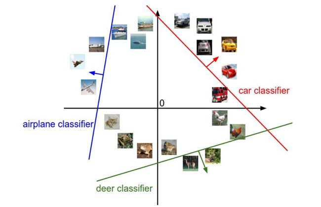
- 将线性分类器看作模板匹配
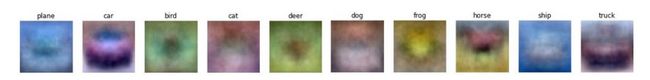
权重 W W W的另一种解释是 W W W的每一行对应于其中一个类的模板(有时也称为原型)。然后,通过使用内积(或点积)将每个模板与图像进行比较,来获得图像的每个类别的分数。
略过一步:在学习CIFAR-10结束时,示例学习了权重。例如,ship模板按预期包含许多蓝色像素。因此,一旦该模板与海洋上的船舶图像相匹配,通过内积运算,它将获得很高的分数。
- Bias trick

- 图像数据预处理:特征缩放 / 均值归一化
损失函数
多类支持向量机(Multiclass SVM)
多类别SVM是在处理多分类问题时的对二元SVM的一种推广。在二元SVM中,只有两个类,每个样本x要么被分类成正例,要么被分类成负例;现在如果有10个类别了,就需要将二元的思想推广到多分类中。
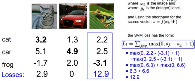
L i = ∑ j ≠ y i max ( 0 , s j − s y i + Δ ) L_i = \sum_{j\neq y_i} \max(0, s_j - s_{y_i} + \Delta) Li=j=yi∑max(0,sj−syi+Δ)
若 Δ = 1 \Delta=1 Δ=1,则:
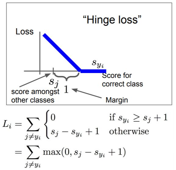
其中, y i y_i yi 表示训练集的第i个样本的真实分类的分数,所以 s y i s_{y_i} syi 表示训练集的第i个样本的真实分类的分数。
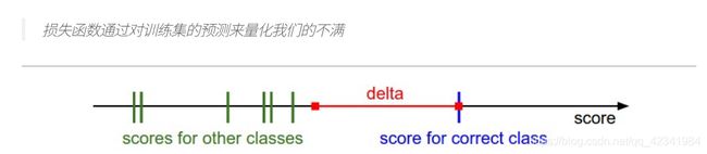
上述公式的理解:
- 如果真实分类的分数比其他分数高很多,这是正确的情况,那要高出多少呢?高出一个安全的边距(这里默认为1)
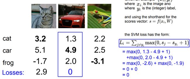
- 如果真实分类的分数不能够比其他分类高出那么多,那就会得到损失,这是不好的情况。
正则化
L = 1 N ∑ i L i ⏟ data loss + λ R ( W ) ⏟ regularization loss L = \underbrace{ \frac{1}{N} \sum_i L_i }_\text{data loss} + \underbrace{ \lambda R(W) }_\text{regularization loss} \\\\ L=data loss N1i∑Li+regularization loss λR(W)
完整形式:
L = 1 N ∑ i ∑ j ≠ y i [ max ( 0 , f ( x i ; W ) j − f ( x i ; W ) y i + Δ ) ] + λ ∑ k ∑ l W k , l 2 L = \frac{1}{N} \sum_i \sum_{j\neq y_i} \left[ \max(0, f(x_i; W)_j - f(x_i; W)_{y_i} + \Delta) \right] + \lambda \sum_k\sum_l W_{k,l}^2 L=N1i∑j=yi∑[max(0,f(xi;W)j−f(xi;W)yi+Δ)]+λk∑l∑Wk,l2

加入正则化项后,决策边界由 f 1 f_1 f1变为 f 2 f_2 f2,惩罚项可以有效防止数据在训练集上过拟合,即趋向“更简单”的模型。
实现过程
def L_i(x, y, W):
  """
  unvectorized version. Compute the multiclass svm loss for a single example (x,y)
  - x is a column vector representing an image (e.g. 3073 x 1 in CIFAR-10)
    with an appended bias dimension in the 3073-rd position (i.e. bias trick)
  - y is an integer giving index of correct class (e.g. between 0 and 9 in CIFAR-10)
  - W is the weight matrix (e.g. 10 x 3073 in CIFAR-10)
  """
  delta = 1.0 # see notes about delta later in this section
  scores = W.dot(x) # scores becomes of size 10 x 1, the scores for each class
  correct_class_score = scores[y]
  D = W.shape[0] # number of classes, e.g. 10
  loss_i = 0.0
  for j in range(D): # iterate over all wrong classes
    if j == y:
      # skip for the true class to only loop over incorrect classes
      continue
    # accumulate loss for the i-th example
    loss_i += max(0, scores[j] - correct_class_score + delta)
  return loss_i

def L_i_vectorized(x, y, W):
  """
  A faster half-vectorized implementation. half-vectorized
  refers to the fact that for a single example the implementation contains
  no for loops, but there is still one loop over the examples (outside this function)
  """
  delta = 1.0
  scores = W.dot(x)
  # compute the margins for all classes in one vector operation
  margins = np.maximum(0, scores - scores[y] + delta)
  # on y-th position scores[y] - scores[y] canceled and gave delta. We want
  # to ignore the y-th position and only consider margin on max wrong class
  margins[y] = 0
  loss_i = np.sum(margins)
  return loss_i

def L(X, y, W):
  """
  fully-vectorized implementation :
  - X holds all the training examples as columns (e.g. 3073 x 50,000 in CIFAR-10)
  - y is array of integers specifying correct class (e.g. 50,000-D array)
  - W are weights (e.g. 10 x 3073)
  """
  # evaluate loss over all examples in X without using any for loops
  # left as exercise to reader in the assignment
Softmax分类器
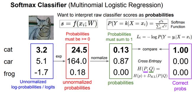
SVM将输出 f ( x i , W ) f(x_i,W) f(xi,W)作为每个类别的分数(未校准且难以解释),而Softmax分类器给出的输出更为直观(标准化的概率)。
首先给出Softmax函数
P ( y i ∣ x i ; W ) = e f y i ∑ j e f j P(y_i \mid x_i; W) = \frac{e^{f_{y_i}}}{\sum_j e^{f_j} } P(yi∣xi;W)=∑jefjefyi
在Softmax中,用交叉熵损失(cross-entropy loss) 代替合页损失(hinge loss):
L i = − log ( e f y i ∑ j e f j ) or equivalently L i = − f y i + log ∑ j e f j L_i = -\log\left(\frac{e^{f_{y_i}}}{ \sum_j e^{f_j} }\right) \hspace{0.5in} \text{or equivalently} \hspace{0.5in} L_i = -f_{y_i} + \log\sum_j e^{f_j} Li=−log(∑jefjefyi)or equivalentlyLi=−fyi+logj∑efj
SVM与Softmax
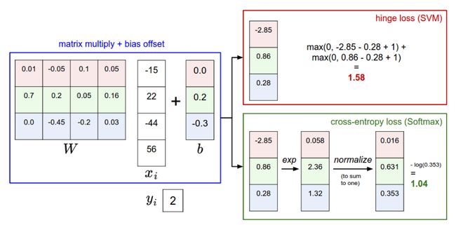
- SVM将这些解释为类别得分,其损失函数鼓励正确的类别(蓝色的class 2)的得分比其他班级的得分高一点。
- Softmax分类器将分数解释为每个类别的(未归一化)对数概率,然后鼓励正确类别的(归一化)对数概率较高(等效地,错误类别较低)。
SVM和Softmax通常是可比较的:
- SVM不在乎单个分数的细节:如果它们分别是[10,-100,-100]或[10,9,9],则由于满足1的裕度,因此SVM不会造成任何损失是零。一旦满足边距,SVM就会很高兴,并且不会对超出这一限制的确切分数进行微管理。
- 但是,对于Softmax分类器,后者会为得分[10,9,9]累积比[10,-100,-100]高得多的损失。换句话说,Softmax分类器对它产生的分数永远不会完全满意:正确的分类总是有较高的概率,而错误的分类总是有较低的概率,损失总是会更好。
优化(Optimization)
计算梯度
有两种计算梯度的方法:一种缓慢,近似但简单的方法(数值梯度),以及一种快速,精确但更容易出错的方法,需要进行演算(解析梯度)。
"""
function : f(x,y,z) = (x+y)z
"""
- 用有限差分数值计算梯度(数值梯度)
# second method  数值法
# increment by epi
def grad2(x,y,z,epi):
    # dx
    fx1 = (x+epi+y)*z
    fx2 = (x-epi+y)*z
    dx = (fx1-fx2)/(2*epi)
    # dy
    fy1 = (x+y+epi)*z
    fy2 = (x+y-epi)*z
    dy = (fy1-fy2)/(2*epi)
    # dz
    fz1 = (x+y)*(z+epi)
    fz2 = (x+y)*(z-epi)
    dz = (fz1-fz2)/(2*epi)
    return (dx,dy,dz)
- 用微积分分析计算梯度(解析梯度)
# first method   解析法
def grad1(x,y,z):
    dx = z
    dy = z
    dz = (x+y)
    return (dx,dy,dz)
梯度下降
重复评估梯度然后执行参数更新的过程称为梯度下降:
# Vanilla Gradient Descent

while True:
  weights_grad = evaluate_gradient(loss_fun, data, weights)
  weights += - step_size * weights_grad # perform parameter update
小批量梯度下降(Mini-batch gradient descent / MBGD),是对批量梯度下降(BGD)以及随机梯度下降(SGD)的一个折中办法。其具体思路是:每次迭代使用 b a t c h s i z e batch_{size} batchsize个样本来对参数进行更新。
这里我们假设 b a t c h s i z e batch_{size} batchsize=10 ,样本数 m=1000 。
伪代码形式为:
repeat{
for i=1,11,21,31,…,991{
θ j : = θ j − α 1 10 ∑ k = i ( i + 9 ) ( h θ ( x ( k ) ) − y ( k ) ) x j ( k ) \theta_j := \theta_j - \alpha \frac{1}{10} \sum_{k=i}^{(i+9)}(h_{\theta}(x^{(k)})-y^{(k)})x_j^{(k)} θj:=θj−α101∑k=i(i+9)(hθ(x(k))−y(k))xj(k)
(for j =0,1)
}
}
例如,在当前最先进的ConvNets中,一个典型的批次包含120万个整个训练集中的256个示例。然后使用该批处理执行参数更新:
# Vanilla Minibatch Gradient Descent

while True:
  data_batch = sample_training_data(data, 256) # sample 256 examples
  weights_grad = evaluate_gradient(loss_fun, data_batch, weights)
  weights += - step_size * weights_grad # perform parameter update
reference
[1]计算梯度的三种方法: 数值法,解析法,反向传播法
[2]批量梯度下降(BGD)、随机梯度下降(SGD)以及小批量梯度下降(MBGD)的理解