python transforms_2.2 图像预处理——transforms(笔记)
目录
任务简介:
熟悉数据预处理transforms方法的运行机制
详细说明:
本节介绍数据的预处理模块transforms的运行机制,数据在读取到pytorch之后通常都需要对数据进行预处理,包括尺寸缩放、转换张量、数据中心化或标准化等等,这些操作都是通过transforms进行的,所以本节重点学习transforms的运行机制并介绍数据标准化(Normalize)的使用原理。
一、transforms运行机制


对图片进行增强的根本原因是为了增强模型的泛化能力。
部分关键代码:
# 训练集的转换
train_transform = transforms.Compose([
transforms.Resize((32, 32)), # 将图片缩放到32 x 32
transforms.RandomCrop(32, padding=4), # 随机裁剪
transforms.ToTensor(), # 将图片转换成张量,同时进行归一化操作,将像素值的区间从0-255归一化到0-1区间。
transforms.Normalize(norm_mean, norm_std), # 数据标准化,将均值变为0,标准差变为1。
])
# 验证集的转换
valid_transform = transforms.Compose([
transforms.Resize((32, 32)),
transforms.ToTensor(),
transforms.Normalize(norm_mean, norm_std),
])
transforms.Compose 是将一系列transforms的方法有序地组合包装,并依次按顺序对数据进行操作,类似于sklearn中的pipline。

二、数据标准化transforms.Normalize()
 数据标准化可以加速模型的收敛。
tensor.sub_()这边下划线表示inplace操作,其余凡有类似下划线情况的均为inplace操作。
逻辑回归测试代码:
import torch
import torch.nn as nn
import matplotlib.pyplot as plt
import numpy as np
torch.manual_seed(10)
lr = 0.01 # 学习率
# 生成虚拟数据
sample_nums = 100
mean_value = 1.7
bias = 5 # 5
n_data = torch.ones(sample_nums, 2)
x0 = torch.normal(mean_value * n_data, 1) + bias # 类别0 数据 shape=(100, 2)
y0 = torch.zeros(sample_nums) # 类别0 标签 shape=(100, 1)
x1 = torch.normal(-mean_value * n_data, 1) + bias # 类别1 数据 shape=(100, 2)
y1 = torch.ones(sample_nums) # 类别1 标签 shape=(100, 1)
train_x = torch.cat((x0, x1), 0)
train_y = torch.cat((y0, y1), 0)
# 定义模型
class LR(nn.Module):
def __init__(self):
super(LR, self).__init__()
self.features = nn.Linear(2, 1)
self.sigmoid = nn.Sigmoid()
def forward(self, x):
x = self.features(x)
x = self.sigmoid(x)
return x
lr_net = LR()
# 定义损失函数与优化器
loss_fn = nn.BCELoss()
optimizer = torch.optim.SGD(lr_net.parameters(), lr=0.01, momentum=0.9)
for iteration in range(1000):
# 前向传播
y_pred = lr_net(train_x)
# 计算 MSE loss
loss = loss_fn(y_pred, train_y)
# 反向传播
loss.backward()
# 更新参数
optimizer.step()
# 清空梯度
optimizer.zero_grad()
# 绘图
if iteration % 40 == 0:
mask = y_pred.ge(0.5).float().squeeze() # 以0.5为阈值进行分类
correct = (mask == train_y).sum() # 计算正确预测的样本个数
acc = correct.item() / train_y.size(0) # 计算精度
plt.scatter(x0.data.numpy()[:, 0], x0.data.numpy()[:, 1], c='r', label='class 0')
plt.scatter(x1.data.numpy()[:, 0], x1.data.numpy()[:, 1], c='b', label='class 1')
w0, w1 = lr_net.features.weight[0]
w0, w1 = float(w0.item()), float(w1.item())
plot_b = float(lr_net.features.bias[0].item())
plot_x = np.arange(-6, 6, 0.1)
plot_y = (-w0 * plot_x - plot_b) / w1
plt.xlim(-5, 10)
plt.ylim(-7, 10)
plt.plot(plot_x, plot_y)
plt.text(-5, 5, 'Loss=%.4f' % loss.data.numpy(), fontdict={'size': 20, 'color': 'red'})
plt.title("Iteration: {}\nw0:{:.2f} w1:{:.2f} b: {:.2f} accuracy:{:.2%}".format(iteration, w0, w1, plot_b, acc))
plt.legend()
plt.show()
plt.pause(0.5)
if acc > 0.99:
break
当bias = 0时,输出:
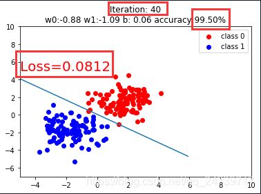
当bias = 5时,输出:

结论:如果训练数据有一个良好的分布和良好的初始化,会加速模型的收敛。
原文链接:https://blog.csdn.net/weixin_40633696/article/details/108027639