NNDL 实验五 前馈神经网络（2）自动梯度计算 & 优化问题

4.3 自动梯度计算和预定义算子

虽然我们能够通过模块化的方式比较好地对神经网络进行组装，但是每个模块的梯度计算过程仍然十分繁琐且容易出错。在深度学习框架中，已经封装了自动梯度计算的功能，我们只需要聚焦模型架构，不再需要耗费精力进行计算梯度。
飞桨提供了paddle.nn.Layer类，来方便快速的实现自己的层和模型。模型和层都可以基于paddle.nn.Layer扩充实现，模型只是一种特殊的层。
继承了paddle.nn.Layer类的算子中，可以在内部直接调用其它继承paddle.nn.Layer类的算子，飞桨框架会自动识别算子中内嵌的paddle.nn.Layer类算子，并自动计算它们的梯度，并在优化时更新它们的参数。

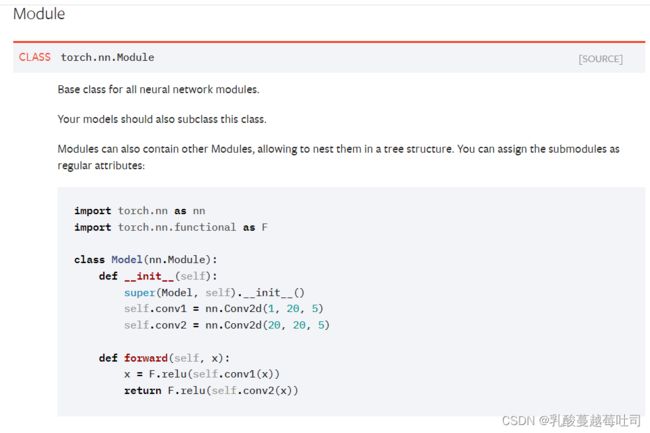
pytorch中的相应内容是什么？请简要介绍。
torch提供了torch.nn.Module类，来方便快速的实现自己的层和模型。模型和层都可以基于nn扩充实现，模型只是一种特殊的层。它继承了torch.nn.Module类的算子中，可以在内部直接调用其它继承的算子，torch框架会自动识别算子中内嵌的torch.nn.Module类算子，并自动计算它们的梯度，并在优化时更新它们的参数。

4.3.1 使用pytorch的预定义算子来重新实现二分类任务

需手动设置w和b。

import torch.nn as nn
import torch.nn.functional as F
import os
import torch
from abc import abstractmethod
import math
import numpy as np

import matplotlib.pyplot as plt
from torch.nn.init  import normal_,constant_,uniform_
class Model_MLP_L2_V2(nn.Module):
    def __init__(self, input_size, hidden_size, output_size):
        super(Model_MLP_L2_V2, self).__init__()
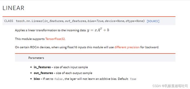
        self.fc1 = nn.Linear(input_size, hidden_size)
        normal_(self.fc1.weight, mean=0., std=1.)
        constant_(self.fc1.bias, val=0.0)
        self.fc2 = nn.Linear(hidden_size, output_size)
        normal_(self.fc2.weight, mean=0., std=1.)
        constant_(self.fc2.bias, val=0.0)
        self.act_fn = torch.sigmoid
    # 前向计算
    def forward(self, inputs):
        z1 = self.fc1(inputs)
        a1 = self.act_fn(z1)
        z2 = self.fc2(a1)
        a2 = self.act_fn(z2)
        return a2

make_moons函数：

import torch
def make_moons(n_samples=1000, shuffle=True, noise=None):
    n_samples_out = n_samples // 2
    n_samples_in = n_samples - n_samples_out
    outer_circ_x = torch.cos(torch.linspace(0, math.pi, n_samples_out))
    outer_circ_y = torch.sin(torch.linspace(0, math.pi, n_samples_out))
    inner_circ_x = 1 - torch.cos(torch.linspace(0, math.pi, n_samples_in))
    inner_circ_y = 0.5 - torch.sin(torch.linspace(0, math.pi, n_samples_in))
    X = torch.stack(
        [torch.cat([outer_circ_x, inner_circ_x]),
         torch.cat([outer_circ_y, inner_circ_y])],
         axis=1
    )
    y = torch.cat(
        [torch.zeros([n_samples_out]), torch.ones([n_samples_in])]
    )
    if shuffle:
        idx = torch.randperm(X.shape[0])
        X = X[idx]
        y = y[idx]
    if noise is not None:
        X += np.random.normal(0.0, noise, X.shape)

    return X, y

accuracy函数：

def accuracy(preds, labels):
    if preds.shape[1] == 1:
        preds=(preds>=0.5).to(torch.float32)

    else:
        preds = torch.argmax(preds,dim=1).int()

    return torch.mean((preds == labels).float())

4.3.2 完善Runner类

class RunnerV2_2(object):
    def __init__(self, model, optimizer, metric, loss_fn, **kwargs):
        self.model = model
        self.optimizer = optimizer
        self.loss_fn = loss_fn
        self.metric = metric

        # 记录训练过程中的评估指标变化情况
        self.train_scores = []
        self.dev_scores = []

        # 记录训练过程中的评价指标变化情况
        self.train_loss = []
        self.dev_loss = []

    def train(self, train_set, dev_set, **kwargs):
        # 将模型切换为训练模式
        self.model.train()

        # 传入训练轮数，如果没有传入值则默认为0
        num_epochs = kwargs.get("num_epochs", 0)
        # 传入log打印频率，如果没有传入值则默认为100
        log_epochs = kwargs.get("log_epochs", 100)
        # 传入模型保存路径，如果没有传入值则默认为"best_model.pdparams"
        save_path = kwargs.get("save_path", "best_model.pdparams")

        # log打印函数，如果没有传入则默认为"None"
        custom_print_log = kwargs.get("custom_print_log", None)

        # 记录全局最优指标
        best_score = 0
        # 进行num_epochs轮训练
        for epoch in range(num_epochs):
            X, y = train_set

            # 获取模型预测
            logits = self.model(X.to(torch.float32))
            # 计算交叉熵损失
            trn_loss = self.loss_fn(logits, y)
            self.train_loss.append(trn_loss.item())
            # 计算评估指标
            trn_score = self.metric(logits, y).item()
            self.train_scores.append(trn_score)

            # 自动计算参数梯度
            trn_loss.backward()
            if custom_print_log is not None:
                # 打印每一层的梯度
                custom_print_log(self)

            # 参数更新
            self.optimizer.step()
            # 清空梯度
            self.optimizer.zero_grad()   # reset gradient

            dev_score, dev_loss = self.evaluate(dev_set)
            # 如果当前指标为最优指标，保存该模型
            if dev_score > best_score:
                self.save_model(save_path)
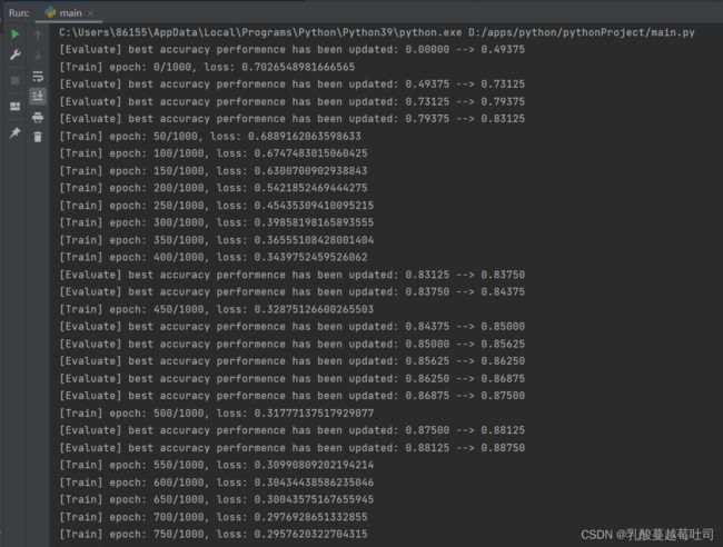
                print(f"[Evaluate] best accuracy performence has been updated: {best_score:.5f} --> {dev_score:.5f}")
                best_score = dev_score

            if log_epochs and epoch % log_epochs == 0:
                print(f"[Train] epoch: {epoch}/{num_epochs}, loss: {trn_loss.item()}")
    @torch.no_grad()
    def evaluate(self, data_set):
        # 将模型切换为评估模式
        self.model.eval()

        X, y = data_set
        # 计算模型输出
        logits = self.model(X)
        # 计算损失函数
        loss = self.loss_fn(logits, y).item()
        self.dev_loss.append(loss)
        # 计算评估指标
        score = self.metric(logits, y).item()
        self.dev_scores.append(score)
        return score, loss

    # 模型测试阶段，使用'torch.no_grad()'控制不计算和存储梯度
    @torch.no_grad()
    def predict(self, X):
        # 将模型切换为评估模式
        self.model.eval()
        return self.model(X)

    # 使用'model.state_dict()'获取模型参数，并进行保存
    def save_model(self, saved_path):
        torch.save(self.model.state_dict(), saved_path)

    # 使用'model.set_state_dict'加载模型参数
    def load_model(self, model_path):
        state_dict = torch.load(model_path)
        self.model.load_state_dict(state_dict)

4.3.3 模型训练

# 设置模型
input_size = 2
hidden_size = 5
output_size = 1
model = Model_MLP_L2_V4(input_size=input_size, hidden_size=hidden_size, output_size=output_size)

# 设置损失函数
loss_fn = F.binary_cross_entropy

# 设置优化器
learning_rate = 0.2 #5e-2
optimizer = torch.optim.SGD(model.parameters(),lr=learning_rate)

# 设置评价指标
metric = accuracy

# 其他参数
epoch = 1000
saved_path = 'best_model.pdparams'

# 实例化RunnerV2类，并传入训练配置
runner = RunnerV2_2(model, optimizer, metric, loss_fn)

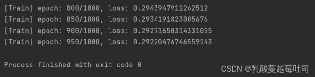
runner.train([X_train, y_train], [X_dev, y_dev], num_epochs = epoch, log_epochs=50, save_path="best_model.pdparams")

结果：


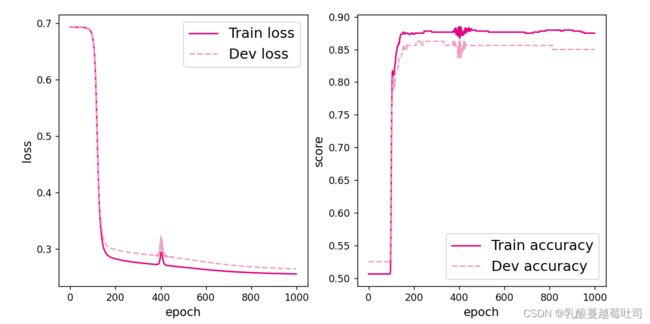
将训练过程中训练集与验证集的准确率变化情况进行可视化。

plot函数:

import matplotlib.pyplot as plt
def plot(runner, fig_name):
    plt.figure(figsize=(10, 5))
    epochs = [i for i in range(len(runner.train_scores))]
 
    plt.subplot(1, 2, 1)
    plt.plot(epochs, runner.train_loss, color='#e4007f', label="Train loss")
    plt.plot(epochs, runner.dev_loss, color='#f19ec2', linestyle='--', label="Dev loss")
    # 绘制坐标轴和图例
    plt.ylabel("loss", fontsize='large')
    plt.xlabel("epoch", fontsize='large')
    plt.legend(loc='upper right', fontsize='x-large')
 
    plt.subplot(1, 2, 2)
    plt.plot(epochs, runner.train_scores, color='#e4007f', label="Train accuracy")
    plt.plot(epochs, runner.dev_scores, color='#f19ec2', linestyle='--', label="Dev accuracy")
    # 绘制坐标轴和图例
    plt.ylabel("score", fontsize='large')
    plt.xlabel("epoch", fontsize='large')
    plt.legend(loc='lower right', fontsize='x-large')
 
    plt.savefig(fig_name)
    plt.show()
 
 
plot(runner, 'fw-acc.pdf')

结果：

4.3.4 性能评价

runner.load_model("best_model.pdparams")
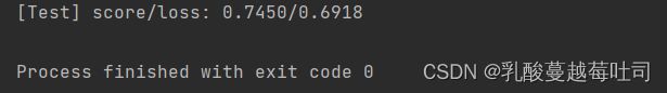
score, loss = runner.evaluate([X_test, y_test])
print("[Test] score/loss: {:.4f}/{:.4f}".format(score, loss))

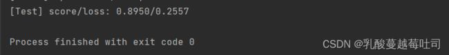
结果：

4.3.5 增加一个3个神经元的隐藏层，再次实现二分类，并与1做对比。（必做）

需做以下改动：

class Model_MLP_L2_V4(torch.nn.Module):
    def __init__(self, input_size, hidden_size, hidden_size2, output_size):
        super(Model_MLP_L2_V4, self).__init__()
        self.fc1 = nn.Linear(input_size, hidden_size)
        w1=torch.normal(0,0.1,size=(hidden_size,input_size),requires_grad=True)
        self.fc1.weight = nn.Parameter(w1)

        self.fc2 = nn.Linear(hidden_size, hidden_size2)
        w2 = torch.normal(0, 0.1, size=(hidden_size2, hidden_size), requires_grad=True)
        self.fc2.weight = nn.Parameter(w2)

        self.fc3 = nn.Linear(hidden_size2, output_size)
        w3 = torch.normal(0, 0.1, size=(output_size, hidden_size2), requires_grad=True)
        self.fc3.weight = nn.Parameter(w3)

        # 使用'torch.nn.functional.sigmoid'定义 Logistic 激活函数
        self.act_fn = torch.sigmoid

    # 前向计算
    def forward(self, inputs):
        z1 = self.fc1(inputs.to(torch.float32))
        a1 = self.act_fn(z1)
        z2 = self.fc2(a1)
        a2 = self.act_fn(z2)
        z3 = self.fc3(a2)
        a3 = self.act_fn(z3)
        return a3

# 设置模型
input_size = 2
hidden_size = 5
hidden_size2 = 3
output_size = 1
model = Model_MLP_L2_V4(input_size=input_size, hidden_size=hidden_size,hidden_size2=hidden_size2, output_size=output_size)

运行了好几次，loss和score都特别不稳定，有点小离谱。比如其中任意两次结果：

根据结果看出，跳不出极小值点，所以我调大学习率为3


发现这个效果一下就上去了，然后又多试了几次：

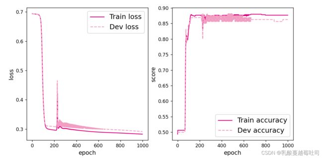
还算是比较稳定的，心满意足了。
通过结果我们可以显著的发现，增加了一层含有三个神经元的隐藏层后，误差和学习率均往好的方面走了！通过调试学习率，使结果也稳定了下来。

4.3.6 自定义隐藏层层数和每个隐藏层中的神经元个数，尝试找到最优超参数完成二分类。可以适当修改数据集，便于探索超参数。（选做）

定义隐藏层层数和神经元个数有些经验之谈。
隐藏层的层数
在神经网络中，当且仅当数据非线性分离时需要隐藏层。对于一般简单的数据集，一两层隐藏层就够了，对于涉及到时间序列和计算机视觉的复杂数据集，需要额外增加层数。单层神经网络只能用于线性分离函数（分类问题中两个类可以用一条直线整齐地分开）。多个隐藏层可以用于拟合非线性函数。隐藏层的层数与神经网络的效果，可以概括为：

• 没有隐藏层（none）：仅能够表示线性可分函数或决策
• 隐藏层数=1：可以拟合任何“包含从一个有限空间到另一个有限空间的连续映射”的函数
• 隐藏层数=2：搭配适当的激活函数可以表示任意精度的任意决策边界，并且可以拟合任何精度的任何平滑映射
• 隐藏层数>2：多出来的隐藏层可以学习复杂的描述（某种自动特征工程）

层数越深，理论上拟合函数的能力增强，效果按理说会更好，但是实际上更深的层数可能会带来过拟合的问题，同时也会增加训练难度，使模型难以收敛。在使用BP神经网络时，最好可以参照已有的表现优异的模型，或者根据上面的表格，从一两层开始尝试，尽量不要使用太多的层数。在CV、NLP等特殊领域，可以使用CNN、RNN、attention等特殊模型，不能不考虑实际而直接无脑堆砌多层神经网络。尝试迁移和微调已有的预训练模型，能取得事半功倍的效果。

隐藏层中神经元数量
隐藏层中使用太少的神经元将导致欠拟合(underfitting)。相反，使用过多的神经元同样会导致一些问题。首先，隐藏层中的神经元过多可能会导致过拟合(overfitting)。当神经网络具有过多的节点（过多的信息处理能力）时，训练集中包含的有限信息量不足以训练隐藏层中的所有神经元，因此就会导致过拟合。即使训练数据包含的信息量足够，隐藏层中过多的神经元会增加训练时间，从而难以达到预期的效果。显然，选择一个合适的隐藏层神经元数量是至关重要的。
通常，对所有隐藏层使用相同数量的神经元就足够了。对于某些数据集，拥有较大的第一层并在其后跟随较小的层将导致更好的性能，因为第一层可以学习很多低阶的特征，这些较低层的特征可以馈入后续层中，提取出较高阶特征。
需要注意的是，与在每一层中添加更多的神经元相比，添加层层数将获得更大的性能提升。因此，不要在一个隐藏层中加入过多的神经元。
如何确定神经元数量，有大神给出了经验以供参考：

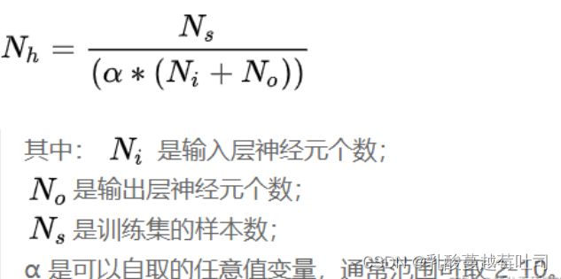
还有一种方法：

• 隐藏神经元的数量应在输入层的大小和输出层的大小之间。
• 隐藏神经元的数量应为输入层大小的2/3加上输出层大小的2/3。
• 隐藏神经元的数量应小于输入层大小的两倍。

隐藏层神经元最佳数量需要通过自己不断试验获得，建议从一个较小的数值比如1到5和1到100个神经元开始，如果欠拟合后会慢慢添加更多的层和神经元，如果过拟合就减小层数和神经元，实际过程中还可以考虑引入Batch Normalization, Dropout, early-stopping、添加正则化项等降低过拟合的方法。

参考文章：确定神经网络的层数和隐藏层的神经元数量

最后我决定隐藏层有一个或者两个，然后进行神经元的设置。上面实验结果发现了学习率太低跳不出局部最小值，下边的都以学习率为3做实验！

先是一个隐藏层5个神经元：

一个隐藏层4个神经元：

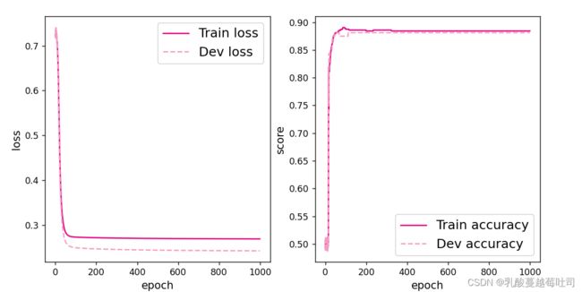
一个隐藏层3个神经元：

这个结果好好呀！惊到我了。然后我决定试试两个隐藏层都是5个神经元：

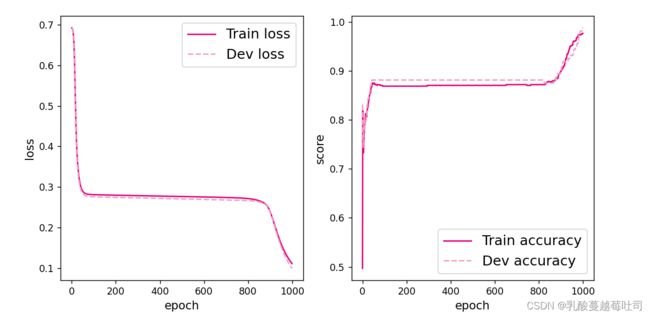
学习率下降了一些，把其中一个隐层的神经元变成3：


这个真的好！考虑到前边一直以学习率为3，现在调一下学习率变为5：

学习率反而下降了。
通过上边，我设置的两个隐层，一个神经元个数为5，另一个为3，学习率为3的参数下，模型性能相对最好。

【思考题】
自定义梯度计算和自动梯度计算：
从计算性能、计算结果等多方面比较，谈谈自己的看法。

pytorch提供的autograd包能够根据输入和前向传播过程自动构建计算图，并执行反向传播。autograd 包是 PyTorch 中所有神经网络的核心。首先让我们简要地介绍它，然后我们将会去训练我们的第一个神经网络。该 autograd 软件包为 Tensors 上的所有操作提供自动微分。它是一个由运行定义的框架，这意味着以代码运行方式定义你的后向传播，并且每次迭代都可以不同。

上次实验，手动计算梯度，得到的模型评价：

本次实验自动梯度计算模型评价：

不难发现自动梯度计算得到的模型效果更好，后向传播的计算部分变成loss.backward()方法，和之前的代码相比更加简洁。并且加入requires_grad=True之后，意味着所有后续跟params相关的调用和操作记录都会被保留下来，任何一个经过params变换得到的新的tensor都可以追踪它的变换记录，如果它的变换函数是可微的，导数的值会被自动放进params的grad属性中。

4.4 优化问题

4.4.1 参数初始化

实现一个神经网络前，需要先初始化模型参数。
如果对每一层的权重和偏置都用0初始化，那么通过第一遍前向计算，所有隐藏层神经元的激活值都相同；在反向传播时，所有权重的更新也都相同，这样会导致隐藏层神经元没有差异性，出现对称权重现象。

将模型参数全都初始化为0：

class Model_MLP_L2_V4(torch.nn.Module):
    def __init__(self, input_size, hidden_size, output_size):
        super(Model_MLP_L2_V4, self).__init__()
        # 使用'torch.nn.Linear'定义线性层。
        # 其中第一个参数（in_features）为线性层输入维度；第二个参数（out_features）为线性层输出维度
        # weight为权重参数属性,bias为偏置参数属性，这里使用'torch.nn.init.constant_'进行常量初始化
        self.fc1 = nn.Linear(input_size, hidden_size)
        constant_(tensor=self.fc1.weight, val=0.0)
        constant_(tensor=self.fc1.bias, val=0.0)
        self.fc2 = nn.Linear(hidden_size, output_size)
        constant_(tensor=self.fc2.weight, val=0.0)
        constant_(tensor=self.fc2.bias, val=0.0)
        # 使用'torch.nn.functional.sigmoid'定义 Logistic 激活函数
        self.act_fn = F.sigmoid

    # 前向计算
    def forward(self, inputs):
        z1 = self.fc1(inputs)
        a1 = self.act_fn(z1)
        z2 = self.fc2(a1)
        a2 = self.act_fn(z2)
        return a2


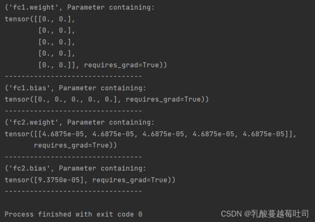
def print_weights(runner):
    print('The weights of the Layers：')

    for _, param in enumerate(runner.model.named_parameters()):
        print(param)

利用Runner类训练模型：

# 设置模型
input_size = 2
hidden_size = 5
output_size = 1
model = Model_MLP_L2_V4(input_size=input_size, hidden_size=hidden_size, output_size=output_size)
 
# 设置损失函数
loss_fn = F.binary_cross_entropy
 
# 设置优化器
learning_rate = 0.2 #5e-2
optimizer = torch.optim.SGD(lr=learning_rate, params=model.parameters())
 
# 设置评价指标
metric = accuracy
 
# 其他参数
epoch = 2000
saved_path = 'best_model.pdparams'
 
# 实例化RunnerV2类，并传入训练配置
runner = RunnerV2_2(model, optimizer, metric, loss_fn)
 
runner.train([X_train, y_train], [X_dev, y_dev], num_epochs=5, log_epochs=50, save_path="best_model.pdparams",custom_print_log=print_weights)

结果：

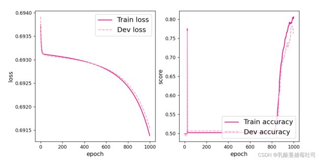
可视化训练和验证集上的主准确率和loss变化：

plot(runner, 'fw-acc.pdf')

从输出结果看，二分类准确率为50%左右，说明模型没有学到任何内容。训练和验证loss几乎没有怎么下降。

为了避免对称权重现象，可以使用高斯分布或均匀分布初始化神经网络的参数。

4.4.2 梯度消失问题

在神经网络的构建过程中，随着网络层数的增加，理论上网络的拟合能力也应该是越来越好的。但是随着网络变深，参数学习更加困难，容易出现梯度消失问题。

由于Sigmoid型函数的饱和性，饱和区的导数更接近于0，误差经过每一层传递都会不断衰减。当网络层数很深时，梯度就会不停衰减，甚至消失，使得整个网络很难训练，这就是所谓的梯度消失问题。
在深度神经网络中，减轻梯度消失问题的方法有很多种，一种简单有效的方式就是使用导数比较大的激活函数，如：ReLU。

4.4.2.1 模型构建

定义一个前馈神经网络，包含4个隐藏层和1个输出层，通过传入的参数指定激活函数。代码实现如下：

# 定义多层前馈神经网络
class Model_MLP_L5(torch.nn.Module):
    def __init__(self, input_size, output_size, act='relu'):
        super(Model_MLP_L5, self).__init__()
        self.fc1 = torch.nn.Linear(input_size, 3)
        w_ = torch.normal(0, 0.01, size=(3, input_size), requires_grad=True)
        self.fc1.weight = nn.Parameter(w_)
        self.fc1.bias = nn.init.constant_(self.fc1.bias, val=1.0)
        w= torch.normal(0, 0.01, size=(3, 3), requires_grad=True)

        self.fc2 = torch.nn.Linear(3, 3)
        self.fc2.weight = nn.Parameter(w)
        self.fc2.bias = nn.init.constant_(self.fc2.bias, val=1.0)
        self.fc3 = torch.nn.Linear(3, 3)
        self.fc3.weight = nn.Parameter(w)
        self.fc3.bias = nn.init.constant_(self.fc3.bias, val=1.0)
        self.fc4 = torch.nn.Linear(3, 3)
        self.fc4.weight = nn.Parameter(w)
        self.fc4.bias = nn.init.constant_(self.fc4.bias, val=1.0)
        self.fc5 = torch.nn.Linear(3, output_size)
        w1 = torch.normal(0, 0.01, size=(output_size, 3), requires_grad=True)
        self.fc5.weight = nn.Parameter(w1)
        self.fc5.bias = nn.init.constant_(self.fc5.bias, val=1.0)
        # 定义网络使用的激活函数
        if act == 'sigmoid':
            self.act = F.sigmoid
        elif act == 'relu':
            self.act = F.relu
        elif act == 'lrelu':
            self.act = F.leaky_relu
        else:
            raise ValueError("Please enter sigmoid relu or lrelu!")


    def forward(self, inputs):
        outputs = self.fc1(inputs.to(torch.float32))
        outputs = self.act(outputs)
        outputs = self.fc2(outputs)
        outputs = self.act(outputs)
        outputs = self.fc3(outputs)
        outputs = self.act(outputs)
        outputs = self.fc4(outputs)
        outputs = self.act(outputs)
        outputs = self.fc5(outputs)
        outputs = F.sigmoid(outputs)
        return outputs

4.4.2.2 使用Sigmoid型函数进行训练

使用Sigmoid型函数作为激活函数，为了便于观察梯度消失现象，只进行一轮网络优化。代码实现如下：

# 学习率大小
lr = 0.01

# 定义网络，激活函数使用sigmoid
model = Model_MLP_L5(input_size=2, output_size=1, act='sigmoid')

# 定义优化器
optimizer = torch.optim.SGD(model.parameters(),lr=lr)

# 定义损失函数，使用交叉熵损失函数
loss_fn = F.binary_cross_entropy

# 定义评价指标
metric = accuracy


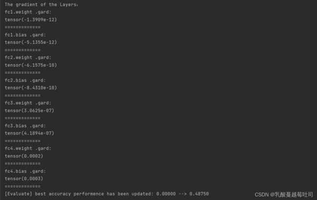
def print_grads(runner):
    # 打印每一层的权重的模
    print('The gradient of the Layers：')
    for item in runner.model.named_parameters():
        if len(item[1])==3:
            print(item[0],".gard:")
            print(torch.mean(item[1].grad))
            print("=============")
# 指定梯度打印函数
custom_print_log = print_grads
# 实例化Runner类
runner = RunnerV2_2(model, optimizer, metric, loss_fn)
# 启动训练
runner.train([X_train, y_train], [X_dev, y_dev],
             num_epochs=1, log_epochs=None,
             save_path="best_model.pdparams",
             custom_print_log=custom_print_log)

结果：

观察得出梯度经过每一个神经层的传递都会不断衰减，最终传递到第一个神经层时，梯度几乎完全消失。

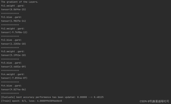
4.4.2.3 使用ReLU函数进行模型训练

torch.manual_seed(102)
# 学习率大小
lr = 0.01

# 定义网络，激活函数使用sigmoid
model = Model_MLP_L5(input_size=2, output_size=1, act='sigmoid')

# 定义优化器
optimizer = torch.optim.SGD(model.parameters(), lr)

# 定义损失函数，使用交叉熵损失函数
loss_fn = F.binary_cross_entropy

# 定义评价指标
metric = accuracy

# 指定梯度打印函数
custom_print_log = print_grads
# 实例化Runner类
runner = RunnerV2_2(model, optimizer, metric, loss_fn)
# 启动训练
runner.train([X_train, y_train], [X_dev, y_dev],
             num_epochs=1, log_epochs=None,
             save_path="best_model.pdparams",
             custom_print_log=custom_print_log)

结果：

4.4.3 死亡ReLU问题

ReLU激活函数可以一定程度上改善梯度消失问题，但是ReLU函数在某些情况下容易出现死亡 ReLU问题，使得网络难以训练。这是由于当x<0时，ReLU函数的输出恒为0。在训练过程中，如果参数在一次不恰当的更新后，某个ReLU神经元在所有训练数据上都不能被激活（即输出为0），那么这个神经元自身参数的梯度永远都会是0，在以后的训练过程中永远都不能被激活。而一种简单有效的优化方式就是将激活函数更换为Leaky ReLU、ELU等ReLU的变种。

4.4.3.1 使用ReLU进行模型训练

# 定义多层前馈神经网络
class Model_MLP_L5(torch.nn.Module):
    def __init__(self, input_size, output_size, act='relu'):
        super(Model_MLP_L5, self).__init__()
        self.fc1 = torch.nn.Linear(input_size, 3)
        w_ = torch.normal(0, 0.01, size=(3, input_size), requires_grad=True)
        self.fc1.weight = nn.Parameter(w_)
        # self.fc1.bias = nn.init.constant_(self.fc1.bias, val=1.0)
        self.fc1.bias = nn.init.constant_(self.fc1.bias, val=-8.0)
        w= torch.normal(0, 0.01, size=(3, 3), requires_grad=True)

        self.fc2 = torch.nn.Linear(3, 3)
        self.fc2.weight = nn.Parameter(w)
        # self.fc2.bias = nn.init.constant_(self.fc2.bias, val=1.0)
        self.fc1.bias = nn.init.constant_(self.fc1.bias, val=-8.0)
        self.fc3 = torch.nn.Linear(3, 3)
        self.fc3.weight = nn.Parameter(w)
        # self.fc3.bias = nn.init.constant_(self.fc2.bias, val=1.0)
        self.fc3.bias = nn.init.constant_(self.fc3.bias, val=-8.0)
        self.fc4 = torch.nn.Linear(3, 3)
        self.fc4.weight = nn.Parameter(w)
        # self.fc4.bias = nn.init.constant_(self.fc2.bias, val=1.0)
        self.fc4.bias = nn.init.constant_(self.fc4.bias, val=-8.0)
        self.fc5 = torch.nn.Linear(3, output_size)
        w1 = torch.normal(0, 0.01, size=(output_size, 3), requires_grad=True)
        self.fc5.weight = nn.Parameter(w1)
        # self.fc5.bias = nn.init.constant_(self.fc2.bias, val=1.0)
        self.fc5.bias = nn.init.constant_(self.fc5.bias, val=-8.0)
        # 定义网络使用的激活函数
        if act == 'sigmoid':
            self.act = F.sigmoid
        elif act == 'relu':
            self.act = F.relu
        elif act == 'lrelu':
            self.act = F.leaky_relu
        else:
            raise ValueError("Please enter sigmoid relu or lrelu!")


    def forward(self, inputs):
        outputs = self.fc1(inputs.to(torch.float32))
        outputs = self.act(outputs)
        outputs = self.fc2(outputs)
        outputs = self.act(outputs)
        outputs = self.fc3(outputs)
        outputs = self.act(outputs)
        outputs = self.fc4(outputs)
        outputs = self.act(outputs)
        outputs = self.fc5(outputs)
        outputs = F.sigmoid(outputs)
        return outputs

结果：

从输出结果可以发现，使用 ReLU 作为激活函数，当满足条件时，会发生死亡ReLU问题，网络训练过程中 ReLU 神经元的梯度始终为0，参数无法更新。针对死亡ReLU问题，一种简单有效的优化方式就是将激活函数更换为Leaky ReLU、ELU等ReLU 的变种。接下来，观察将激活函数更换为 Leaky ReLU时的梯度情况。

4.4.3.2 使用Leaky ReLU进行模型训练

# 定义网络，激活函数使用sigmoid
model = Model_MLP_L5(input_size=2, output_size=1, act='lrelu')


# 实例化Runner类
runner = RunnerV2_2(model, optimizer, metric, loss_fn)

# 启动训练
runner.train([X_train, y_train], [X_dev, y_dev], 
            num_epochs=1, log_epochps=None, 
            save_path="best_model.pdparams", 
            custom_print_log=custom_print_log)

结果：

从输出结果可以看到，将激活函数更换为Leaky ReLU后，死亡ReLU问题得到了改善，梯度恢复正常，参数也可以正常更新。但是由于 Leaky ReLU 中，x<0 时的斜率默认只有0.01，所以反向传播时，随着网络层数的加深，梯度值越来越小。如果想要改善这一现象，将 Leaky ReLU 中，x<0 时的斜率调大即可。

总结：看了同学的博客知道了一个更全的pytorch和paddle的转换关系，在初始化模型的时候也会注意到不同的小细节。
通过自定义隐层和对应的神经元数量，这个调参的过程让我直观的感受了一下参数不同对模型性能的影响，但看其他同学博客还对噪声进行了调参，希望下次能深刻的理解一下这个参数。