第七章图像处理

7.1
f = imread(“F:\picture files\Fig0524(b)(blurred-impulse).tif”);
w = [-1 -1 -1;-1 8 -1;-1 -1 -1]; % 点检测掩模
g = abs(imfilter(double(f),w));
T = max(g();
g = g>=T;
subplot(1,2,1);imshow(f);title(’(a)原图像’);
subplot(1,2,2);imshow(g);title(’(b)点检测’);

7.2
f = imread(“D:\tp\DIP3E_Original_Images_CH09\Fig0905(a)(wirebond-mask).tif”); % 图像大小：486×486
w = [2 -1 -1;-1 2 -1;-1 -1 2]; % +45°方向检测线
g = imfilter(double(f),w);
gtop = g(1:120,1:120); % 左上角区域
gtop = pixeldup(gtop,4); % 通过复制像素将图像扩大gtop*4倍
gbot = g(end-119:end,end-119:end); % 右下角区域
gbot = pixeldup(gbot,4);
g1 = abs(g); % 检测图的绝对值
T = max(g1();
g2 = g1>=T;

subplot(3,2,1);imshow(f);title(’(a)连线模板图像’);
subplot(3,2,2);imshow(g,[]);title(’(b)+45°线处理后的结果’);
subplot(3,2,3);imshow(gtop,[]);title(‘©(b)中左上角的放大效果’);
subplot(3,2,4);imshow(gbot,[]);title(’(d)(b)中右下角的放大效果’);
subplot(3,2,5);imshow(g1,[]);title(’(e)(b)的绝对值’);
subplot(3,2,6);imshow(g2);title(’(f)满足g>=T的所有点’);
7.3
f = imread(“D:\DIP3E_Original_Images_CH04\Fig0438(a)(bld_600by600).tif”); % 图像大小：486×486
subplot(3,2,1),imshow(f),title(’(a)原始图像’);
[gv, t] = edge(f,‘sobel’,‘vertical’);
subplot(3,2,2),imshow(gv),title(’(b)Sobel模板处理后结果’);
gv = edge(f, ‘sobel’, 0.15, ‘vertical’);
subplot(3,2,3),imshow(gv),title(‘©使用指定阈值的结果’);
gboth = edge(f, ‘sobel’, 0.15);
subplot(3,2,4),imshow(gboth),title(’(d)指点阈值确定垂直边缘和水平边缘的结果’);
w45 = [-2 -1 0;-1 0 1; 0 1 2];
g45 = imfilter(double(f), w45, ‘replicate’);
T = 0.3 * max(abs(g45());
g45 = g45 >= T;
subplot(3,2,5),imshow(g45),title(’(e)-45°方向边缘’);
f45= [0 1 2;-1 0 1;-2 -1 0];
h45= imfilter(double(f), f45,‘replicate’);
T = 0.3 * max(abs(h45());
h45 = h45 >= T;
subplot(3,2,6),imshow(h45),title(’(f)+45°方向边缘’);
7.4
f=imread(‘E:\PICTRUE\Fig0438(a)(bld_600by600).tif’);
f=tofloat(f);
F=fft2(f);
S=fftshift(log(1+abs(F)));
imshow(S,[ ])

h=fspecial(‘sobel’)
freqz2(h)
PQ=paddedsize(size(f));
H=freqz2(h,PQ(1),PQ(2));
H1=ifftshift(H);

imshow(abs(H),[ ])
figure,imshow(abs(H1),[ ])

gs=imfilter(f,h);
gf=dftfilt(f,H1);
imshow(gs,[ ])
figure,imshow(gf,[ ])
figure,imshow(abs(gs),[ ])
figure,imshow(abs(gf),[ ])
figure,imshow(abs(gs)>0.2*abs(max(gs()))
figure,imshow(abs(gf)>0.abs(max(gf()))

7.5
clc;
clear;
f=imread(‘E:\PICTRUE\Fig0441(a)(characters_test_pattern).tif’);
[f,revertclass]=tofloat(f);
PQ=paddedsize(size(f));
[U,V]=dftuv(PQ(1),PQ(2));
D=hypot(U,V);
D0=0.05PQ(2);
F=fft2(f,PQ(1),PQ(2));
H=exp(-(D.^2)/(2*(D02)));
g=dftfilt(f,H);
g=revertclass(g);
figure
subplot(221);imshow(f);title(‘ԭʼͼÏñ’);
subplot(222);imshow(fftshift(H));title(‘ÒÔͼÏñÏÔʾµÄ¸ß˹µÍͨÂ˲¨Æ÷’);
subplot(223);imshow(log(1+abs(fftshift(F))),[]);title(‘Â˲¨Ç°Í¼ÏñµÄÆ×’);
subplot(224);imshow(g);title(‘Â˲¨ºóµÄͼÏñ’);

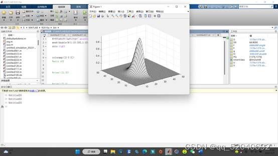
7.6
H=fftshift(lpfilter(‘gaussian’,500,500,50));
mesh(double(H(1:10:500,1:10:500)));
axis tight

colormap([0 0 0])
axis off

view(-25,30)

view(-25,0)

7.7
H=fftshift(hpfilter(‘gaussian’,500,500,50));
mesh(double(H(1:10:500,1:10:500)));
axis tight
colormap([0 0 0])
axis off
figure,imshow(H,[ ])

H=fftshift(hpfilter(‘ideal’,500,500,50));
mesh(double(H(1:10:500,1:10:500)));
axis tight
colormap([0 0 0])
axis off
figure,imshow(H,[ ])

7.8
f=imread(‘E:\PICTRUE\Fig0441(a)(characters_test_pattern).tif’);
PQ=paddedsize(size(f));
D0=0.05PQ(1);
imshow(f);title(‘ԭʼͼÏñ’);
H=hpfilter(‘gaussian’,PQ(1),PQ(2),D0);
g=dftfilt(f,H);
figure,imshow(g)
7.9
I1=imread(‘E:\PICTRUE\Fig0459(a)(orig_chest_xray).tif’);
[len,wed]=size(I1);
g=fft2(I1);
g=fftshift(g);
[M,N]=size(g);
m=fix(M/2);
n=fix(N/2);
D0=40;
n1=2
for i=1:M
for j=1:N
D=sqrt((i-m)^2+(j-n)2);
H1=1-exp((-1)(D^2/(2*D02)));
H2=0.5+0.75H1;%¸ù¾Ý¸ø¶¨µÄk1\k2Á½¸öϵÊý¶Ô´«µÝº¯Êý½øÐÐÐÞ¸Ä
s1(i,j)=H1g(i,j);
s2(i,j)=H2*g(i,j);%¸ßƵǿµ÷Â˲¨ÊÇÀûÓÃÐ޸ĺóµÄº¯Êý½øÐÐƵÓòÏà³Ë
end
end
I2=im2uint8(real(ifft2(ifftshift(s1)/255)));
I3=im2uint8(real(ifft2(ifftshift(s2)/255)));
I4=histeq(I3);%¸ßƵǿµ÷Â˲¨ÔöÇ¿ºÍÖ±·½Í¼¾ùºâ»¯Êdz£¼ûµÄ´îÅä´¦Àí·½Ê½£¬¿ÉÒԵõ½¸üºÃµÄͼÏñЧ¹û
subplot(221),imshow(I1),title(‘ԭͼ’);
subplot(222),imshow(I2),title(‘¸ß˹¸ßƵÂ˲¨Í¼’);
subplot(223),imshow(I3),title(‘¸ß˹¸ßƵǿµ÷Â˲¨Í¼’);
subplot(224),imshow(I4),title(‘Ö±·½Í¼¾ùºâ»¯’);

7.10
f = tofloat(imread(“D:\tp\DIP3E_Original_Images_CH10\Fig1043(a)(yeast_USC).tif”));
subplot(2,2,1),imshow(f);title(’(a) 酵母细胞的图像’);
[TGlobal] = graythresh(f);
gGlobal = im2bw(f, TGlobal);
subplot(2,2,2),imshow(gGlobal);title(’(b)用 Otsus 方法分割的图像’);
g = localthresh(f, ones(3), 30, 1.5, ‘global’);
SIG = stdfilt(f, ones(3));
subplot(2,2,3), imshow(SIG, [ ]) ;title(‘© 局部标准差图像’);
subplot(2,2,4),imshow(g);title(’(d) 用局部阈值处理分割的图像 ‘);
7.11
f = imread(“C:\Users\桦仔\Desktop\冈萨雷斯《数字图像处理》（MATLAB版）电子版、图源、代码\课本原图片\DIP3E_Original_Images_CH06\Fig0621(a)(weld-original).tif”);
subplot(2,2,1),imshow(f);
title(’(a)显示有焊接缺陷的图像’);
%函数regiongrow返回的NR为是不同区域的数目，参数SI是一副含有种子点的图像
%TI是包含在经过连通前通过阈值测试的像素
[g,NR,SI,TI]=regiongrow(f,1,0.26);%种子的像素值为255，65为阈值
subplot(2,2,2),imshow(SI);
title(’(b)种子点’);
subplot(2,2,3),imshow(TI);
title(‘©通过了阈值测试的像素的二值图像(白色)’);
subplot(2,2,4),imshow(g);
title(’(d)对种子点进行8连通分析后的结果’);
7.12

f = imread(“C:\Users\桦仔\Desktop\冈萨雷斯《数字图像处理》（MATLAB版）电子版、图源、代码\课本原图片\DIP3E_Original_Images_CH06\Fig0621(a)(weld-original).tif”);
subplot(2,2,1),imshow(f);
title(’(a)显示有焊接缺陷的图像’);
%函数regiongrow返回的NR为是不同区域的数目，参数SI是一副含有种子点的图像
%TI是包含在经过连通前通过阈值测试的像素
[g,NR,SI,TI]=regiongrow(f,1,0.26);%种子的像素值为255，65为阈值
subplot(2,2,2),imshow(SI);
title(’(b)种子点’);
subplot(2,2,3),imshow(TI);
title(‘©通过了阈值测试的像素的二值图像(白色)’);
subplot(2,2,4),imshow(g);
title(’(d)对种子点进行8连通分析后的结果’);