Assignment | 02-week2 -Optimization Methods
该系列仅在原课程基础上课后作业部分添加个人学习笔记,或相关推导补充等。如有错误,还请批评指教。在学习了 Andrew Ng 课程的基础上,为了更方便的查阅复习,将其整理成文字。因本人一直在学习英语,所以该系列以英文为主,同时也建议读者以英文为主,中文辅助,以便后期进阶时,为学习相关领域的学术论文做铺垫。- ZJ
Coursera 课程 |deeplearning.ai |网易云课堂
转载请注明作者和出处:ZJ 微信公众号-「SelfImprovementLab」
知乎:https://zhuanlan.zhihu.com/c_147249273
CSDN:http://blog.csdn.net/junjun_zhao/article/details/79125104
Until now, you’ve always used Gradient Descent to update the parameters and minimize the cost. In this notebook, you will learn more advanced optimization methods that can speed up learning and perhaps even get you to a better final value for the cost function. Having a good optimization algorithm can be the difference between waiting days vs. just a few hours to get a good result.
Gradient descent goes “downhill” on a cost function J J . Think of it as trying to do this:

At each step of the training, you update your parameters following a certain direction to try to get to the lowest possible point.
Notations: As usual, ∂J∂a= ∂ J ∂ a = da for any variable a.
To get started, run the following code to import the libraries you will need.
import numpy as np
import matplotlib.pyplot as plt
import scipy.io
import math
import sklearn
import sklearn.datasets

from opt_utils import load_params_and_grads, initialize_parameters, forward_propagation, backward_propagation
from opt_utils import compute_cost, predict, predict_dec, plot_decision_boundary, load_dataset
from testCases import *

%matplotlib inline
plt.rcParams['figure.figsize'] = (7.0, 4.0) # set default size of plots
plt.rcParams['image.interpolation'] = 'nearest'
plt.rcParams['image.cmap'] = 'gray'
1 - Gradient Descent
A simple optimization method in machine learning is gradient descent (GD). When you take gradient steps with respect to all m m examples on each step, it is also called Batch Gradient Descent.
Warm-up exercise: Implement the gradient descent update rule. The gradient descent rule is, for l=1,...,L l = 1 , . . . , L :
where L is the number of layers and α α is the learning rate. All parameters should be stored in the parameters dictionary. Note that the iterator l starts at 0 in the for loop while the first parameters are W[1] W [ 1 ] and b[1] b [ 1 ] . You need to shift l to l+1 when coding.
# GRADED FUNCTION: update_parameters_with_gd

def update_parameters_with_gd(parameters, grads, learning_rate):
    """
    Update parameters using one step of gradient descent

    Arguments:
    parameters -- python dictionary containing your parameters to be updated:
                    parameters['W' + str(l)] = Wl
                    parameters['b' + str(l)] = bl
    grads -- python dictionary containing your gradients to update each parameters:
                    grads['dW' + str(l)] = dWl
                    grads['db' + str(l)] = dbl
    learning_rate -- the learning rate, scalar.

    Returns:
    parameters -- python dictionary containing your updated parameters
    """

    L = len(parameters) // 2 # number of layers in the neural networks

    # Update rule for each parameter
    for l in range(L):
        ### START CODE HERE ### (approx. 2 lines)
        parameters["W" + str(l+1)] = parameters["W" + str(l+1)] - learning_rate * grads['dW' + str(l+1)]
        parameters["b" + str(l+1)] = parameters["b" + str(l+1)] - learning_rate * grads['db' + str(l+1)]
        ### END CODE HERE ###

    return parameters

#  错误点 :parameters["W" + str(l+1)] - learning_rate * grads['dW' + str(l+1)]
#  没有 W0
parameters, grads, learning_rate = update_parameters_with_gd_test_case()
parameters = update_parameters_with_gd(parameters, grads, learning_rate)
print("W1 = " + str(parameters["W1"]))
print("b1 = " + str(parameters["b1"]))
print("W2 = " + str(parameters["W2"]))
print("b2 = " + str(parameters["b2"]))W1 = [[ 1.63535156 -0.62320365 -0.53718766]
[-1.07799357 0.85639907 -2.29470142]]
b1 = [[ 1.74604067]
[-0.75184921]]
W2 = [[ 0.32171798 -0.25467393 1.46902454]
[-2.05617317 -0.31554548 -0.3756023 ]
[ 1.1404819 -1.09976462 -0.1612551 ]]
b2 = [[-0.88020257]
[ 0.02561572]
[ 0.57539477]]
Expected Output:
| **W1** | [[ 1.63535156 -0.62320365 -0.53718766] [-1.07799357 0.85639907 -2.29470142]] |
| **b1** | [[ 1.74604067] [-0.75184921]] |
| **W2** | [[ 0.32171798 -0.25467393 1.46902454] [-2.05617317 -0.31554548 -0.3756023 ] [ 1.1404819 -1.09976462 -0.1612551 ]] |
| **b2** | [[-0.88020257] [ 0.02561572] [ 0.57539477]] |
A variant of this is Stochastic Gradient Descent (SGD) 随机梯度, which is equivalent 等同于 to mini-batch gradient descent where each mini-batch has just 1 example. The update rule that you have just implemented does not change. What changes is that you would be computing gradients on just one training example at a time, rather than on the whole training set. The code examples below illustrate the difference between stochastic gradient descent and (batch) gradient descent.
- (Batch) Gradient Descent: 一次处理所有数据 只有一个for循环 迭代次数
X = data_input
Y = labels
parameters = initialize_parameters(layers_dims)
for i in range(0, num_iterations):
    # Forward propagation
    a, caches = forward_propagation(X, parameters)
    # Compute cost.
    cost = compute_cost(a, Y)
    # Backward propagation.
    grads = backward_propagation(a, caches, parameters)
    # Update parameters.
    parameters = update_parameters(parameters, grads)
- Stochastic Gradient Descent: SGD 随机梯度下降 一次处理一个数据,等同于 mini-batch has just 1 example 三层 for 循环 m 个样本 和迭代次数 和层数 1- l
X = data_input
Y = labels
parameters = initialize_parameters(layers_dims)
for i in range(0, num_iterations):
    for j in range(0, m):
        # Forward propagation
        a, caches = forward_propagation(X[:,j], parameters)
        # Compute cost
        cost = compute_cost(a, Y[:,j])
        # Backward propagation
        grads = backward_propagation(a, caches, parameters)
        # Update parameters.
        parameters = update_parameters(parameters, grads)
In Stochastic Gradient Descent, you use only 1 training example before updating the gradients. When the training set is large, SGD can be faster. But the parameters will “oscillate” 震荡 波动大 toward the minimum rather than converge smoothly.而不是收敛的相对平滑 Here is an illustration of this:

“+” denotes a minimum of the cost. SGD leads to many oscillations to reach convergence. But each step is a lot faster to compute for SGD than for GD, as it uses only one training example (vs. the whole batch for GD).
Note also that implementing SGD requires 3 for-loops in total:
1. Over the number of iterations
2. Over the m m training examples
3. Over the layers (to update all parameters, from (W[1],b[1]) ( W [ 1 ] , b [ 1 ] ) to (W[L],b[L]) ( W [ L ] , b [ L ] ) )
In practice, you’ll often get faster results if you do not use neither the whole training set, nor only one training example, to perform each update. Mini-batch gradient descent uses an intermediate number of examples for each step. With mini-batch gradient descent, you loop over the mini-batches instead of looping over individual training examples.
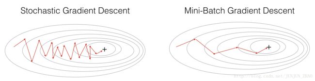
“+” denotes a minimum of the cost. Using mini-batches in your optimization algorithm often leads to faster optimization.
What you should remember:
- The difference between gradient descent, mini-batch gradient descent and stochastic gradient descent is the number of examples you use to perform one update step. GD mini-batch GD 和 SGD 之间的区别是执行更新时,样本数目的不同
- You have to tune a learning rate hyperparameter α α .
- With a well-turned mini-batch size, usually it outperforms either gradient descent or stochastic gradient descent (particularly when the training set is large). 一个调整很好的 mini-batch 大小的参数,通常比其他的 GD or SGD 都表现的效果梗好,尤其是在训练集非常大的情况下。
2 - Mini-Batch Gradient descent
Let’s learn how to build mini-batches from the training set (X, Y).
There are two steps:
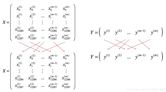
- Shuffle: Create a shuffled version of the training set (X, Y) as shown below. Each column of X and Y represents a training example. Note that the random shuffling is done synchronously between X and Y. Such that after the shuffling the ith i t h column of X is the example corresponding to the ith i t h label in Y. The shuffling step ensures that examples will be split randomly into different mini-batches.
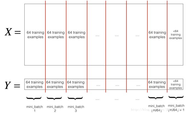
- Partition: Partition the shuffled (X, Y) into mini-batches of size
mini_batch_size(here 64). Note that the number of training examples is not always divisible bymini_batch_size. The last mini batch might be smaller, but you don’t need to worry about this. When the final mini-batch is smaller than the fullmini_batch_size, it will look like this:
Exercise: Implement random_mini_batches. We coded the shuffling part for you. To help you with the partitioning step, we give you the following code that selects the indexes for the 1st 1 s t and 2nd 2 n d mini-batches:
first_mini_batch_X = shuffled_X[:, 0 : mini_batch_size]
second_mini_batch_X = shuffled_X[:, mini_batch_size : 2 * mini_batch_size]
...
Note that the last mini-batch might end up smaller than mini_batch_size=64. Let ⌊s⌋ ⌊ s ⌋ represents s s rounded down to the nearest integer (this is math.floor(s) in Python). If the total number of examples is not a multiple of mini_batch_size=64 then there will be ⌊mmini_batch_size⌋ ⌊ m m i n i _ b a t c h _ s i z e ⌋ mini-batches with a full 64 examples, and the number of examples in the final mini-batch will be ( m−mini_batch_size×⌊mmini_batch_size⌋ m − m i n i _ b a t c h _ s i z e × ⌊ m m i n i _ b a t c h _ s i z e ⌋ ).
# GRADED FUNCTION: random_mini_batches

def random_mini_batches(X, Y, mini_batch_size = 64, seed = 0):
    """
    Creates a list of random minibatches from (X, Y)

    Arguments:
    X -- input data, of shape (input size, number of examples)
    Y -- true "label" vector (1 for blue dot / 0 for red dot), of shape (1, number of examples)
    mini_batch_size -- size of the mini-batches, integer

    Returns:
    mini_batches -- list of synchronous (mini_batch_X, mini_batch_Y)
    """

    np.random.seed(seed)            # To make your "random" minibatches the same as ours
    m = X.shape[1]                  # number of training examples
    mini_batches = []

    # Step 1: Shuffle (X, Y)
    permutation = list(np.random.permutation(m))
    shuffled_X = X[:, permutation]
    shuffled_Y = Y[:, permutation].reshape((1,m))

    # Step 2: Partition (shuffled_X, shuffled_Y). Minus the end case.
    # math.floor 下取整
    num_complete_minibatches = math.floor(m/mini_batch_size) # number of mini batches of size mini_batch_size in your partitionning
    for k in range(0, num_complete_minibatches):
        ### START CODE HERE ### (approx. 2 lines)
        mini_batch_X = shuffled_X[:, k * mini_batch_size : (k+1) * mini_batch_size]
        mini_batch_Y = shuffled_Y[:, k * mini_batch_size : (k+1) * mini_batch_size]
        ### END CODE HERE ###
        mini_batch = (mini_batch_X, mini_batch_Y)
        mini_batches.append(mini_batch)

    # Handling the end case (last mini-batch < mini_batch_size)
    if m % mini_batch_size != 0:
        ### START CODE HERE ### (approx. 2 lines)
        mini_batch_X = shuffled_X[:, mini_batch_size * num_complete_minibatches : m ]
        mini_batch_Y = shuffled_Y[:, mini_batch_size * num_complete_minibatches : m ]
        ### END CODE HERE ###
        mini_batch = (mini_batch_X, mini_batch_Y)
        mini_batches.append(mini_batch)

    return mini_batches
X_assess, Y_assess, mini_batch_size = random_mini_batches_test_case()
mini_batches = random_mini_batches(X_assess, Y_assess, mini_batch_size)
print ("shape of the 1st mini_batch_X: " + str(mini_batches[0][0].shape))
print ("shape of the 2nd mini_batch_X: " + str(mini_batches[1][0].shape))
print ("shape of the 3rd mini_batch_X: " + str(mini_batches[2][0].shape))
print ("shape of the 1st mini_batch_Y: " + str(mini_batches[0][1].shape))
print ("shape of the 2nd mini_batch_Y: " + str(mini_batches[1][1].shape))
print ("shape of the 3rd mini_batch_Y: " + str(mini_batches[2][1].shape))
print ("mini batch sanity check: " + str(mini_batches[0][0][0][0:3]))shape of the 1st mini_batch_X: (12288, 64)
shape of the 2nd mini_batch_X: (12288, 64)
shape of the 3rd mini_batch_X: (12288, 20)
shape of the 1st mini_batch_Y: (1, 64)
shape of the 2nd mini_batch_Y: (1, 64)
shape of the 3rd mini_batch_Y: (1, 20)
mini batch sanity check: [ 0.90085595 -0.7612069 0.2344157 ]
Expected Output:
| **shape of the 1st mini_batch_X** | (12288, 64) |
| **shape of the 2nd mini_batch_X** | (12288, 64) |
| **shape of the 3rd mini_batch_X** | (12288, 20) |
| **shape of the 1st mini_batch_Y** | (1, 64) |
| **shape of the 2nd mini_batch_Y** | (1, 64) |
| **shape of the 3rd mini_batch_Y** | (1, 20) |
| **mini batch sanity check** | [ 0.90085595 -0.7612069 0.2344157 ] |
What you should remember:
- Shuffling and Partitioning are the two steps required to build mini-batches Shuffling and Partitioning 是建立 mini-batches 所需要的两个步骤
- Powers of two are often chosen to be the mini-batch size, e.g., 16, 32, 64, 128. 大小通常是 2 的 次方
3 - Momentum
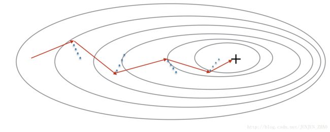
Because mini-batch gradient descent makes a parameter update after seeing just a subset of examples, the direction of the update has some variance, and so the path taken by mini-batch gradient descent will “oscillate” toward convergence.收敛 Using momentum can reduce these oscillations.振荡
Momentum takes into account the past gradients to smooth out the update. We will store the ‘direction’ of the previous gradients in the variable v v . Formally, this will be the exponentially weighted average of the gradient on previous steps. You can also think of v v as the “velocity” 速度 of a ball rolling downhill, building up speed (and momentum) 加速度according to the direction of the gradient/slope of the hill.
Exercise: Initialize the velocity. The velocity, v v , is a python dictionary that needs to be initialized with arrays of zeros. Its keys are the same as those in the grads dictionary, that is:
for l=1,...,L l = 1 , . . . , L :
v["dW" + str(l+1)] = ... #(numpy array of zeros with the same shape as parameters["W" + str(l+1)])
v["db" + str(l+1)] = ... #(numpy array of zeros with the same shape as parameters["b" + str(l+1)])
Note that the iterator l starts at 0 in the for loop while the first parameters are v[“dW1”] and v[“db1”] (that’s a “one” on the superscript). This is why we are shifting l to l+1 in the for loop.
# GRADED FUNCTION: initialize_velocity

def initialize_velocity(parameters):
    """
    Initialize the velocity. The velocity,  vv , is a python dictionary that needs to be initialized with arrays of zeros.
    初始化 速度,0 矩阵 形状和 w 的形状是一样的
    Initializes the velocity as a python dictionary with:
                - keys: "dW1", "db1", ..., "dWL", "dbL"
                - values: numpy arrays of zeros of the same shape as the corresponding gradients/parameters.
    Arguments:
    parameters -- python dictionary containing your parameters.
                    parameters['W' + str(l)] = Wl
                    parameters['b' + str(l)] = bl

    Returns:
    v -- python dictionary containing the current velocity.
                    v['dW' + str(l)] = velocity of dWl
                    v['db' + str(l)] = velocity of dbl
    """

    L = len(parameters) // 2 # number of layers in the neural networks
    v = {}

    # Initialize velocity
    for l in range(L):
        ### START CODE HERE ### (approx. 2 lines)
        v["dW" + str(l+1)] = np.zeros(parameters['W' + str(l+1)].shape)
        v["db" + str(l+1)] = np.zeros(parameters['b' + str(l+1)].shape)
        ### END CODE HERE ###

    return v
parameters = initialize_velocity_test_case()
v = initialize_velocity(parameters)
print("v[\"dW1\"] = " + str(v["dW1"]))
print("v[\"db1\"] = " + str(v["db1"]))
print("v[\"dW2\"] = " + str(v["dW2"]))
print("v[\"db2\"] = " + str(v["db2"]))v["dW1"] = [[0. 0. 0.]
[0. 0. 0.]]
v["db1"] = [[0.]
[0.]]
v["dW2"] = [[0. 0. 0.]
[0. 0. 0.]
[0. 0. 0.]]
v["db2"] = [[0.]
[0.]
[0.]]
Expected Output:
| **v[“dW1”]** | [[ 0. 0. 0.] [ 0. 0. 0.]] |
| **v[“db1”]** | [[ 0.] [ 0.]] |
| **v[“dW2”]** | [[ 0. 0. 0.] [ 0. 0. 0.] [ 0. 0. 0.]] |
| **v[“db2”]** | [[ 0.] [ 0.] [ 0.]] |
Exercise: Now, implement the parameters update with momentum. The momentum update rule is, for l=1,...,L l = 1 , . . . , L :
where L is the number of layers, β β is the momentum 动量 and α α is the learning rate. All parameters should be stored in the parameters dictionary. Note that the iterator l starts at 0 in the for loop while the first parameters are W[1] W [ 1 ] and b[1] b [ 1 ] (that’s a “one” on the superscript). So you will need to shift l to l+1 when coding.
# GRADED FUNCTION: update_parameters_with_momentum
def update_parameters_with_momentum(parameters, grads, v, beta, learning_rate):
"""
Update parameters using Momentum
Arguments:
parameters -- python dictionary containing your parameters:
parameters['W' + str(l)] = Wl
parameters['b' + str(l)] = bl
grads -- python dictionary containing your gradients for each parameters:
grads['dW' + str(l)] = dWl
grads['db' + str(l)] = dbl
v -- python dictionary containing the current velocity:
v['dW' + str(l)] = ...
v['db' + str(l)] = ...
beta -- the momentum hyperparameter, scalar
learning_rate -- the learning rate, scalar
Returns:
parameters -- python dictionary containing your updated parameters
v -- python dictionary containing your updated velocities
"""
L = len(parameters) // 2 # number of layers in the neural networks
# Momentum update for each parameter
for l in range(L):
### START CODE HERE ### (approx. 4 lines)
# compute velocities
v["dW" + str(l+1)] = beta * v['dW' + str(l+1)] + (1 - beta)* grads['dW' + str(l+1)]
v["db" + str(l+1)] = beta * v['db' + str(l+1)] + (1 - beta)* grads['db' + str(l+1)]
# update parameters
parameters["W" + str(l+1)] = parameters['W' + str(l+1)] - learning_rate * v["dW" + str(l+1)]
parameters["b" + str(l+1)] = parameters['b' + str(l+1)] - learning_rate * v["db" + str(l+1)]
### END CODE HERE ###
return parameters, vparameters, grads, v = update_parameters_with_momentum_test_case()
parameters, v = update_parameters_with_momentum(parameters, grads, v, beta = 0.9, learning_rate = 0.01)
print("W1 = " + str(parameters["W1"]))
print("b1 = " + str(parameters["b1"]))
print("W2 = " + str(parameters["W2"]))
print("b2 = " + str(parameters["b2"]))
print("v[\"dW1\"] = " + str(v["dW1"]))
print("v[\"db1\"] = " + str(v["db1"]))
print("v[\"dW2\"] = " + str(v["dW2"]))
print("v[\"db2\"] = " + str(v["db2"]))W1 = [[ 1.62544598 -0.61290114 -0.52907334]
[-1.07347112 0.86450677 -2.30085497]]
b1 = [[ 1.74493465]
[-0.76027113]]
W2 = [[ 0.31930698 -0.24990073 1.4627996 ]
[-2.05974396 -0.32173003 -0.38320915]
[ 1.13444069 -1.0998786 -0.1713109 ]]
b2 = [[-0.87809283]
[ 0.04055394]
[ 0.58207317]]
v["dW1"] = [[-0.11006192 0.11447237 0.09015907]
[ 0.05024943 0.09008559 -0.06837279]]
v["db1"] = [[-0.01228902]
[-0.09357694]]
v["dW2"] = [[-0.02678881 0.05303555 -0.06916608]
[-0.03967535 -0.06871727 -0.08452056]
[-0.06712461 -0.00126646 -0.11173103]]
v["db2"] = [[0.02344157]
[0.16598022]
[0.07420442]]
Expected Output:
| **W1** | [[ 1.62544598 -0.61290114 -0.52907334] [-1.07347112 0.86450677 -2.30085497]] |
| **b1** | [[ 1.74493465] [-0.76027113]] |
| **W2** | [[ 0.31930698 -0.24990073 1.4627996 ] [-2.05974396 -0.32173003 -0.38320915] [ 1.13444069 -1.0998786 -0.1713109 ]] |
| **b2** | [[-0.87809283] [ 0.04055394] [ 0.58207317]] |
| **v[“dW1”]** | [[-0.11006192 0.11447237 0.09015907] [ 0.05024943 0.09008559 -0.06837279]] |
| **v[“db1”]** | [[-0.01228902] [-0.09357694]] |
| **v[“dW2”]** | [[-0.02678881 0.05303555 -0.06916608] [-0.03967535 -0.06871727 -0.08452056] [-0.06712461 -0.00126646 -0.11173103]] |
| **v[“db2”]** | [[ 0.02344157] [ 0.16598022] [ 0.07420442]] |
Note that:
- The velocity is initialized with zeros. So the algorithm will take a few iterations to “build up” velocity and start to take bigger steps.
- If β=0 β = 0 , then this just becomes standard gradient descent without momentum.
How do you choose β β ?
- The larger the momentum β β is, the smoother the update because the more we take the past gradients into account. But if β β is too big, it could also smooth out the updates too much.
- Common values for β β range from 0.8 to 0.999. If you don’t feel inclined to tune this, β=0.9 β = 0.9 is often a reasonable default.
- Tuning the optimal β β for your model might need trying several values to see what works best in term of reducing the value of the cost function J J .
What you should remember:
- Momentum takes past gradients into account to smooth out the steps of gradient descent. It can be applied with batch gradient descent, mini-batch gradient descent or stochastic gradient descent.
- You have to tune a momentum hyperparameter β β and a learning rate α α .
4 - Adam
Adam is one of the most effective optimization algorithms for training neural networks. It combines ideas from RMSProp (described in lecture) and Momentum.
How does Adam work?
1. It calculates an exponentially weighted average of past gradients, and stores it in variables v v (before bias correction) and vcorrected v c o r r e c t e d (with bias correction).
2. It calculates an exponentially weighted average of the squares of the past gradients, and stores it in variables s s (before bias correction) and scorrected s c o r r e c t e d (with bias correction).
3. It updates parameters in a direction based on combining information from “1” and “2”.
The update rule is, for l=1,...,L l = 1 , . . . , L :
where:
- t counts the number of steps taken of Adam
- L is the number of layers
- β1 β 1 and β2 β 2 are hyperparameters that control the two exponentially weighted averages.
- α α is the learning rate
- ε ε is a very small number to avoid dividing by zero
As usual, we will store all parameters in the parameters dictionary
Exercise: Initialize the Adam variables v,s v , s which keep track of the past information.
Instruction: The variables v,s v , s are python dictionaries that need to be initialized with arrays of zeros. Their keys are the same as for grads, that is:
for l=1,...,L l = 1 , . . . , L :
v["dW" + str(l+1)] = ... #(numpy array of zeros with the same shape as parameters["W" + str(l+1)])
v["db" + str(l+1)] = ... #(numpy array of zeros with the same shape as parameters["b" + str(l+1)])
s["dW" + str(l+1)] = ... #(numpy array of zeros with the same shape as parameters["W" + str(l+1)])
s["db" + str(l+1)] = ... #(numpy array of zeros with the same shape as parameters["b" + str(l+1)])
# GRADED FUNCTION: initialize_adam
def initialize_adam(parameters) :
"""
Initializes v and s as two python dictionaries with:
- keys: "dW1", "db1", ..., "dWL", "dbL"
- values: numpy arrays of zeros of the same shape as the corresponding gradients/parameters.
Arguments:
parameters -- python dictionary containing your parameters.
parameters["W" + str(l)] = Wl
parameters["b" + str(l)] = bl
Returns:
v -- python dictionary that will contain the exponentially weighted average of the gradient.
v["dW" + str(l)] = ...
v["db" + str(l)] = ...
s -- python dictionary that will contain the exponentially weighted average of the squared gradient.
s["dW" + str(l)] = ...
s["db" + str(l)] = ...
"""
L = len(parameters) // 2 # number of layers in the neural networks
v = {}
s = {}
# Initialize v, s. Input: "parameters". Outputs: "v, s".
for l in range(L):
### START CODE HERE ### (approx. 4 lines)
v["dW" + str(l+1)] = np.zeros((parameters['W' + str(l+1)].shape[0], parameters['W' + str(l+1)].shape[1]))
v["db" + str(l+1)] = np.zeros((parameters['b' + str(l+1)].shape[0], parameters['b' + str(l+1)].shape[1]))
s["dW" + str(l+1)] = np.zeros((parameters['W' + str(l+1)].shape[0], parameters['W' + str(l+1)].shape[1]))
s["db" + str(l+1)] = np.zeros((parameters['b' + str(l+1)].shape[0], parameters['b' + str(l+1)].shape[1]))
### END CODE HERE ###
return v, sparameters = initialize_adam_test_case()
v, s = initialize_adam(parameters)
print("v[\"dW1\"] = " + str(v["dW1"]))
print("v[\"db1\"] = " + str(v["db1"]))
print("v[\"dW2\"] = " + str(v["dW2"]))
print("v[\"db2\"] = " + str(v["db2"]))
print("s[\"dW1\"] = " + str(s["dW1"]))
print("s[\"db1\"] = " + str(s["db1"]))
print("s[\"dW2\"] = " + str(s["dW2"]))
print("s[\"db2\"] = " + str(s["db2"]))
v["dW1"] = [[0. 0. 0.]
 [0. 0. 0.]]
v["db1"] = [[0.]
 [0.]]
v["dW2"] = [[0. 0. 0.]
 [0. 0. 0.]
 [0. 0. 0.]]
v["db2"] = [[0.]
 [0.]
 [0.]]
s["dW1"] = [[0. 0. 0.]
[0. 0. 0.]]
s["db1"] = [[0.]
[0.]]
s["dW2"] = [[0. 0. 0.]
[0. 0. 0.]
[0. 0. 0.]]
s["db2"] = [[0.]
[0.]
[0.]]
Expected Output:
| **v[“dW1”]** | [[ 0. 0. 0.] [ 0. 0. 0.]] |
| **v[“db1”]** | [[ 0.] [ 0.]] |
| **v[“dW2”]** | [[ 0. 0. 0.] [ 0. 0. 0.] [ 0. 0. 0.]] |
| **v[“db2”]** | [[ 0.] [ 0.] [ 0.]] |
| **s[“dW1”]** | [[ 0. 0. 0.] [ 0. 0. 0.]] |
| **s[“db1”]** | [[ 0.] [ 0.]] |
| **s[“dW2”]** | [[ 0. 0. 0.] [ 0. 0. 0.] [ 0. 0. 0.]] |
| **s[“db2”]** | [[ 0.] [ 0.] [ 0.]] |
Exercise: Now, implement the parameters update with Adam. Recall the general update rule is, for l=1,...,L l = 1 , . . . , L :
Note that the iterator l starts at 0 in the for loop while the first parameters are W[1] W [ 1 ] and b[1] b [ 1 ] . You need to shift l to l+1 when coding.
# GRADED FUNCTION: update_parameters_with_adam

def update_parameters_with_adam(parameters, grads, v, s, t, learning_rate = 0.01,
                                beta1 = 0.9, beta2 = 0.999,  epsilon = 1e-8):
    """
    Update parameters using Adam

    Arguments:
    parameters -- python dictionary containing your parameters:
                    parameters['W' + str(l)] = Wl
                    parameters['b' + str(l)] = bl
    grads -- python dictionary containing your gradients for each parameters:
                    grads['dW' + str(l)] = dWl
                    grads['db' + str(l)] = dbl
    v -- Adam variable, moving average of the first gradient, python dictionary
    s -- Adam variable, moving average of the squared gradient, python dictionary
    learning_rate -- the learning rate, scalar.
    beta1 -- Exponential decay hyperparameter for the first moment estimates
    beta2 -- Exponential decay hyperparameter for the second moment estimates
    epsilon -- hyperparameter preventing division by zero in Adam updates

    Returns:
    parameters -- python dictionary containing your updated parameters
    v -- Adam variable, moving average of the first gradient, python dictionary
    s -- Adam variable, moving average of the squared gradient, python dictionary
    """

    L = len(parameters) // 2                 # number of layers in the neural networks
    v_corrected = {}                         # Initializing first moment estimate, python dictionary
    s_corrected = {}                         # Initializing second moment estimate, python dictionary

    # Perform Adam update on all parameters
    for l in range(L):
        # Moving average of the gradients. Inputs: "v, grads, beta1". Output: "v".
        ### START CODE HERE ### (approx. 2 lines)
        v["dW" + str(l+1)] = beta1 * v["dW" + str(l+1)] + (1-beta1) * grads['dW' + str(l+1)]
        v["db" + str(l+1)] = beta1 * v["db" + str(l+1)] + (1-beta1) * grads['db' + str(l+1)]
        ### END CODE HERE ###

        # Compute bias-corrected first moment estimate. Inputs: "v, beta1, t". Output: "v_corrected".
        ### START CODE HERE ### (approx. 2 lines)
        v_corrected["dW" + str(l+1)] = v["dW" + str(l+1)]/(1-np.power(beta1,t))
        v_corrected["db" + str(l+1)] = v["db" + str(l+1)]/(1-np.power(beta1,t))
        ### END CODE HERE ###

        # Moving average of the squared gradients. Inputs: "s, grads, beta2". Output: "s".
        ### START CODE HERE ### (approx. 2 lines)
        s["dW" + str(l+1)] = beta2 * s["dW" + str(l+1)] + (1-beta2) * np.power(grads['dW' + str(l+1)],2)
        s["db" + str(l+1)] = beta2 * s["db" + str(l+1)] + (1-beta2) * np.power(grads['db' + str(l+1)],2)
        ### END CODE HERE ###

        # Compute bias-corrected second raw moment estimate. Inputs: "s, beta2, t". Output: "s_corrected".
        ### START CODE HERE ### (approx. 2 lines)
        s_corrected["dW" + str(l+1)] = s["dW" + str(l+1)]/(1-np.power(beta2,t))
        s_corrected["db" + str(l+1)] = s["db" + str(l+1)]/(1-np.power(beta2,t))
        ### END CODE HERE ###

        # Update parameters. Inputs: "parameters, learning_rate, v_corrected, s_corrected, epsilon". Output: "parameters".
        ### START CODE HERE ### (approx. 2 lines)
        parameters["W" + str(l+1)] = parameters["W" + str(l+1)] - learning_rate * v_corrected["dW" + str(l+1)]/(np.sqrt(s_corrected["dW" + str(l+1)])+epsilon)
        parameters["b" + str(l+1)] = parameters["b" + str(l+1)] - learning_rate * v_corrected["db" + str(l+1)]/(np.sqrt(s_corrected["db" + str(l+1)])+epsilon)
        ### END CODE HERE ###
# 错误点: +epsilon 因为没有加 +epsilon 所以一直 nan  nan  nan
    return parameters, v, s
parameters, grads, v, s = update_parameters_with_adam_test_case()
parameters, v, s = update_parameters_with_adam(parameters, grads, v, s, t = 2)
print("W1 = " + str(parameters["W1"]))
print("b1 = " + str(parameters["b1"]))
print("W2 = " + str(parameters["W2"]))
print("b2 = " + str(parameters["b2"]))
print("v[\"dW1\"] = " + str(v["dW1"]))
print("v[\"db1\"] = " + str(v["db1"]))
print("v[\"dW2\"] = " + str(v["dW2"]))
print("v[\"db2\"] = " + str(v["db2"]))
print("s[\"dW1\"] = " + str(s["dW1"]))
print("s[\"db1\"] = " + str(s["db1"]))
print("s[\"dW2\"] = " + str(s["dW2"]))
print("s[\"db2\"] = " + str(s["db2"]))W1 = [[ 1.63178673 -0.61919778 -0.53561312]
[-1.08040999 0.85796626 -2.29409733]]
b1 = [[ 1.75225313]
[-0.75376553]]
W2 = [[ 0.32648046 -0.25681174 1.46954931]
[-2.05269934 -0.31497584 -0.37661299]
[ 1.14121081 -1.09244991 -0.16498684]]
b2 = [[-0.88529979]
[ 0.03477238]
[ 0.57537385]]
v["dW1"] = [[-0.11006192 0.11447237 0.09015907]
[ 0.05024943 0.09008559 -0.06837279]]
v["db1"] = [[-0.01228902]
[-0.09357694]]
v["dW2"] = [[-0.02678881 0.05303555 -0.06916608]
[-0.03967535 -0.06871727 -0.08452056]
[-0.06712461 -0.00126646 -0.11173103]]
v["db2"] = [[0.02344157]
[0.16598022]
[0.07420442]]
s["dW1"] = [[0.00121136 0.00131039 0.00081287]
[0.0002525 0.00081154 0.00046748]]
s["db1"] = [[1.51020075e-05]
[8.75664434e-04]]
s["dW2"] = [[7.17640232e-05 2.81276921e-04 4.78394595e-04]
[1.57413361e-04 4.72206320e-04 7.14372576e-04]
[4.50571368e-04 1.60392066e-07 1.24838242e-03]]
s["db2"] = [[5.49507194e-05]
[2.75494327e-03]
[5.50629536e-04]]
Expected Output:
| **W1** | [[ 1.63178673 -0.61919778 -0.53561312] [-1.08040999 0.85796626 -2.29409733]] |
| **b1** | [[ 1.75225313] [-0.75376553]] |
| **W2** | [[ 0.32648046 -0.25681174 1.46954931] [-2.05269934 -0.31497584 -0.37661299] [ 1.14121081 -1.09245036 -0.16498684]] |
| **b2** | [[-0.88529978] [ 0.03477238] [ 0.57537385]] |
| **v[“dW1”]** | [[-0.11006192 0.11447237 0.09015907] [ 0.05024943 0.09008559 -0.06837279]] |
| **v[“db1”]** | [[-0.01228902] [-0.09357694]] |
| **v[“dW2”]** | [[-0.02678881 0.05303555 -0.06916608] [-0.03967535 -0.06871727 -0.08452056] [-0.06712461 -0.00126646 -0.11173103]] |
| **v[“db2”]** | [[ 0.02344157] [ 0.16598022] [ 0.07420442]] |
| **s[“dW1”]** | [[ 0.00121136 0.00131039 0.00081287] [ 0.0002525 0.00081154 0.00046748]] |
| **s[“db1”]** | [[ 1.51020075e-05] [ 8.75664434e-04]] |
| **s[“dW2”]** | [[ 7.17640232e-05 2.81276921e-04 4.78394595e-04] [ 1.57413361e-04 4.72206320e-04 7.14372576e-04] [ 4.50571368e-04 1.60392066e-07 1.24838242e-03]] |
| **s[“db2”]** | [[ 5.49507194e-05] [ 2.75494327e-03] [ 5.50629536e-04]] |
You now have three working optimization algorithms (mini-batch gradient descent, Momentum, Adam). Let’s implement a model with each of these optimizers and observe the difference.
5 - Model with different optimization algorithms
Lets use the following “moons” dataset to test the different optimization methods. (The dataset is named “moons” because the data from each of the two classes looks a bit like a crescent-shaped moon.)
train_X, train_Y = load_dataset()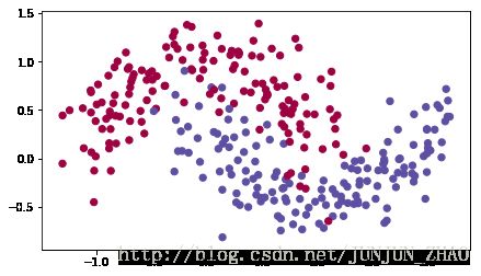
We have already implemented a 3-layer neural network. You will train it with:
- Mini-batch Gradient Descent: it will call your function:
- update_parameters_with_gd()
- Mini-batch Momentum: it will call your functions:
- initialize_velocity() and update_parameters_with_momentum()
- Mini-batch Adam: it will call your functions:
- initialize_adam() and update_parameters_with_adam()
def model(X, Y, layers_dims, optimizer, learning_rate = 0.0007, mini_batch_size = 64, beta = 0.9,
beta1 = 0.9, beta2 = 0.999, epsilon = 1e-8, num_epochs = 10000, print_cost = True):
"""
3-layer neural network model which can be run in different optimizer modes.
Arguments:
X -- input data, of shape (2, number of examples)
Y -- true "label" vector (1 for blue dot / 0 for red dot), of shape (1, number of examples)
layers_dims -- python list, containing the size of each layer
learning_rate -- the learning rate, scalar.
mini_batch_size -- the size of a mini batch
beta -- Momentum hyperparameter
beta1 -- Exponential decay hyperparameter for the past gradients estimates
beta2 -- Exponential decay hyperparameter for the past squared gradients estimates
epsilon -- hyperparameter preventing division by zero in Adam updates
num_epochs -- number of epochs
print_cost -- True to print the cost every 1000 epochs
Returns:
parameters -- python dictionary containing your updated parameters
"""
L = len(layers_dims) # number of layers in the neural networks
costs = [] # to keep track of the cost
t = 0 # initializing the counter required for Adam update
seed = 10 # For grading purposes, so that your "random" minibatches are the same as ours
# Initialize parameters
parameters = initialize_parameters(layers_dims)
# Initialize the optimizer
if optimizer == "gd":
pass # no initialization required for gradient descent
elif optimizer == "momentum":
v = initialize_velocity(parameters)
elif optimizer == "adam":
v, s = initialize_adam(parameters)
# Optimization loop
for i in range(num_epochs):
# Define the random minibatches. We increment the seed to reshuffle differently the dataset after each epoch
seed = seed + 1
minibatches = random_mini_batches(X, Y, mini_batch_size, seed)
for minibatch in minibatches:
# Select a minibatch
(minibatch_X, minibatch_Y) = minibatch
# Forward propagation
a3, caches = forward_propagation(minibatch_X, parameters)
# Compute cost
cost = compute_cost(a3, minibatch_Y)
# Backward propagation
grads = backward_propagation(minibatch_X, minibatch_Y, caches)
# Update parameters
if optimizer == "gd":
parameters = update_parameters_with_gd(parameters, grads, learning_rate)
elif optimizer == "momentum":
parameters, v = update_parameters_with_momentum(parameters, grads, v, beta, learning_rate)
elif optimizer == "adam":
t = t + 1 # Adam counter
parameters, v, s = update_parameters_with_adam(parameters, grads, v, s,
t, learning_rate, beta1, beta2, epsilon)
# Print the cost every 1000 epoch
if print_cost and i % 1000 == 0:
print ("Cost after epoch %i: %f" %(i, cost))
if print_cost and i % 100 == 0:
costs.append(cost)
# plot the cost
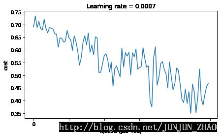
plt.plot(costs)
plt.ylabel('cost')
plt.xlabel('epochs (per 100)')
plt.title("Learning rate = " + str(learning_rate))
plt.show()
return parametersYou will now run this 3 layer neural network with each of the 3 optimization methods.
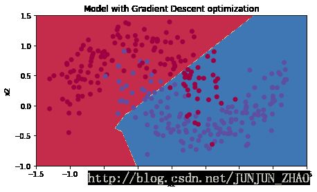
5.1 - Mini-batch Gradient descent
Run the following code to see how the model does with mini-batch gradient descent.
# train 3-layer model
layers_dims = [train_X.shape[0], 5, 2, 1]
parameters = model(train_X, train_Y, layers_dims, optimizer = "gd")

# Predict
predictions = predict(train_X, train_Y, parameters)

# Plot decision boundary
plt.title("Model with Gradient Descent optimization")
axes = plt.gca()
axes.set_xlim([-1.5,2.5])
axes.set_ylim([-1,1.5])
plot_decision_boundary(lambda x: predict_dec(parameters, x.T), train_X, train_Y)
Cost after epoch 0: 0.690736
Cost after epoch 1000: 0.685273
Cost after epoch 2000: 0.647072
Cost after epoch 3000: 0.619525
Cost after epoch 4000: 0.576584
Cost after epoch 5000: 0.607243
Cost after epoch 6000: 0.529403
Cost after epoch 7000: 0.460768
Cost after epoch 8000: 0.465586
Cost after epoch 9000: 0.464518

Accuracy: 0.7966666666666666
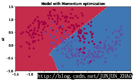
5.2 - Mini-batch gradient descent with momentum
Run the following code to see how the model does with momentum. Because this example is relatively simple, the gains from using momemtum are small; but for more complex problems you might see bigger gains.
# train 3-layer model
layers_dims = [train_X.shape[0], 5, 2, 1]
parameters = model(train_X, train_Y, layers_dims, beta = 0.9, optimizer = "momentum")

# Predict
predictions = predict(train_X, train_Y, parameters)

# Plot decision boundary
plt.title("Model with Momentum optimization")
axes = plt.gca()
axes.set_xlim([-1.5,2.5])
axes.set_ylim([-1,1.5])
plot_decision_boundary(lambda x: predict_dec(parameters, x.T), train_X, train_Y)
Cost after epoch 0: 0.690741
Cost after epoch 1000: 0.685341
Cost after epoch 2000: 0.647145
Cost after epoch 3000: 0.619594
Cost after epoch 4000: 0.576665
Cost after epoch 5000: 0.607324
Cost after epoch 6000: 0.529476
Cost after epoch 7000: 0.460936
Cost after epoch 8000: 0.465780
Cost after epoch 9000: 0.464740
Accuracy: 0.7966666666666666
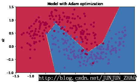
5.3 - Mini-batch with Adam mode
Run the following code to see how the model does with Adam.
# train 3-layer model

layers_dims = [train_X.shape[0], 5, 2, 1]
parameters = model(train_X, train_Y, layers_dims, beta = 0.9,  optimizer = "adam")

# Predict
predictions = predict(train_X, train_Y, parameters)

# Plot decision boundary
plt.title("Model with Adam optimization")
axes = plt.gca()
axes.set_xlim([-1.5,2.5])
axes.set_ylim([-1,1.5])
plot_decision_boundary(lambda x: predict_dec(parameters, x.T), train_X, train_Y)
Cost after epoch 0: 0.690552
Cost after epoch 1000: 0.185567
Cost after epoch 2000: 0.150852
Cost after epoch 3000: 0.074454
Cost after epoch 4000: 0.125936
Cost after epoch 5000: 0.104235
Cost after epoch 6000: 0.100552
Cost after epoch 7000: 0.031601
Cost after epoch 8000: 0.111709
Cost after epoch 9000: 0.197648

Accuracy: 0.94
5.4 - Summary
| **optimization method** | **accuracy** | **cost shape** |
| Gradient descent | 79.7% | oscillations |
| Momentum | 79.7% | oscillations |
| Adam | 94% | smoother |
Momentum usually helps, but given the small learning rate and the simplistic dataset, its impact is almost negligeable. Also, the huge oscillations you see in the cost come from the fact that some minibatches are more difficult thans others for the optimization algorithm.
Adam on the other hand, clearly outperforms mini-batch gradient descent and Momentum. If you run the model for more epochs on this simple dataset, all three methods will lead to very good results. However, you’ve seen that Adam converges a lot faster.
Momentum一般都是有助于提升速度,但是当学习率较小,数据集相对简单的时候,其性能的优越性没有太明显。我们在优化算法中看到的那些较大的震荡是由于一些 minibatches 相对更加复杂所造成的。
从运行结果可以看出,Adam 算法比mini-batch gradient descent 和 Momentum都要显得优越。对于model如果在简单数据集上,迭代次数更多的话,这三种优化算法都会产生较好的结果,但是我们也可以看出,Adam算法收敛得更快些。
Adam算法的优点:
内存要求低 (尽管比gradient descent 和 gradient descent with momentum要高些)
一般微调超参数就可以获得较好的结果(除了α)
Some advantages of Adam include:
- Relatively low memory requirements (though higher than gradient descent and gradient descent with momentum)
- Usually works well even with little tuning of hyperparameters (except α α )
补两个 gif

References:
- Adam paper: https://arxiv.org/pdf/1412.6980.pdf
PS: 欢迎扫码关注公众号:「SelfImprovementLab」!专注「深度学习」,「机器学习」,「人工智能」。以及 「早起」,「阅读」,「运动」,「英语 」「其他」不定期建群 打卡互助活动。
