量子搜索算法基础: Quantum Amplititude Amplification

1. Introduction

You have likely heard that one of the many advantages a quantum computer has over a classical computer is its superior speed searching databases. Grover’s algorithm demonstrates this capability. This algorithm can speed up an unstructured search problem quadratically, but its uses extend beyond that; it can serve as a general trick or subroutine to obtain quadratic run time improvements for a variety of other algorithms. This is called the amplitude amplification trick.

两步走：1. 反转目标状态的振幅；2. 根据平均值再翻转。

2. Unstructured Search

Suppose you are given a large list of N items. Among these items there is one item with a unique property that we wish to locate; we will call this one the winner w. Think of each item in the list as a box of a particular color. Say all items in the list are gray except the winner w, which is purple.

To find the purple box – the marked item – using classical computation, one would have to check on average N/2 of these boxes, and in the worst case, all N of them. On a quantum computer, however, we can find the marked item in roughly \sqrt{N} steps with Grover’s amplitude amplification trick. A quadratic speedup is indeed a substantial time-saver for finding marked items in long lists. Additionally, the algorithm does not use the list’s internal structure, which makes it generic; this is why it immediately provides a quadratic quantum speed-up for many classical problems.

3. Creating an Oracle

For the examples in this textbook, our ‘database’ is comprised of all the possible computational basis states our qubits can be in. For example, if we have 3 qubits, our list is the states |000\rangle, |001\rangle, \dots |111\rangle (i.e the states |0\rangle \rightarrow |7\rangle).

Grover’s algorithm solves oracles that add a negative phase to the solution states. I.e. for any state $|x⟩$ in the computational basis:

$$U_{\omega }|x⟩=\{\begin{array}{r}|x⟩\text{if}x\ne \omega \\ -|x⟩\text{if}x=\omega \end{array}$$
This oracle will be a diagonal matrix, where the entry that correspond to the marked item will have a negative phase. For example, if we have three qubits and \omega = \text{101}, our oracle will have the matrix:

$$U_{\omega }=\left[\begin{array}{cccccccc}1& 0& 0& 0& 0& 0& 0& 0\\ 0& 1& 0& 0& 0& 0& 0& 0\\ 0& 0& 1& 0& 0& 0& 0& 0\\ 0& 0& 0& 1& 0& 0& 0& 0\\ 0& 0& 0& 0& 1& 0& 0& 0\\ 0& 0& 0& 0& 0& -1& 0& 0\\ 0& 0& 0& 0& 0& 0& 1& 0\\ 0& 0& 0& 0& 0& 0& 0& 1\end{array}\right]\begin{array}{r}\\ \\ \\ \\ \\ \\ \leftarrow \omega =\text{101}\\ \\ \\ \end{array}$$

What makes Grover’s algorithm so powerful is how easy it is to convert a problem to an oracle of this form. There are many computational problems in which it’s difficult to find a solution, but relatively easy to verify a solution. For example, we can easily verify a solution to a sudoku by checking all the rules are satisfied. For these problems, we can create a function f that takes a proposed solution x, and returns f(x) = 0 if x is not a solution $(x\ne \omega )$ and f(x) = 1 for a valid solution $(x=\omega )$. Our oracle can then be described as:

$$U_{\omega }|x⟩=(-1{)}^{f(x)}|x⟩$$
and the oracle’s matrix will be a diagonal matrix of the form:

$$U_{\omega }=\left[\begin{array}{cccc}(-1{)}^{f(0)}& 0& \cdots & 0\\ 0& (-1{)}^{f(1)}& \cdots & 0\\ ⋮& 0& \ddots & ⋮\\ 0& 0& \cdots & (-1{)}^{f(2^n-1)}\end{array}\right]$$

For the next part of this chapter, we aim to teach the core concepts of the algorithm. We will create example oracles where we know \omega beforehand, and not worry ourselves with whether these oracles are useful or not. At the end of the chapter, we will cover a short example where we create an oracle to solve a problem (sudoku).

4. Amplitude Amplification

So how does the algorithm work? Before looking at the list of items, we have no idea where the marked item is. Therefore, any guess of its location is as good as any other, which can be expressed in terms of a uniform superposition: $|s⟩=\frac{1}{\sqrt{N}}{\sum }_{x=0}^{N-1}|x⟩$.

If at this point we were to measure in the standard basis $\{|x⟩\}$, this superposition would collapse, according to the fifth quantum law, to any one of the basis states with the same probability of $\frac{1}{N}=\frac{1}{2^n}$. Our chances of guessing the right value w is therefore 1 in $2^n$, as could be expected. Hence, on average we would need to try about $N/2=2^{n-1}$ times to guess the correct item.

Enter the procedure called amplitude amplification, which is how a quantum computer significantly enhances this probability. This procedure stretches out (amplifies) the amplitude of the marked item, which shrinks the other items’ amplitude, so that measuring the final state will return the right item with near-certainty.

This algorithm has a nice geometrical interpretation in terms of two reflections, which generate a rotation in a two-dimensional plane. The only two special states we need to consider are the winner $|w⟩$ and the uniform superposition $|s⟩$. These two vectors span a two-dimensional plane in the vector space ${\mathbb{C}}^N$. They are not quite perpendicular because $|w⟩$ occurs in the superposition with amplitude $N^{-1/2}$ as well. We can, however, introduce an additional state |s’\rangle that is in the span of these two vectors, which is perpendicular to $|w⟩$ and is obtained from $|s⟩$ by removing $|w⟩$ and rescaling.

Step 1: The amplitude amplification procedure starts out in the uniform superposition $|s⟩$, which is easily constructed from $|s⟩=H^{\otimes n}|0{⟩}^n$.

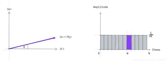
The left graphic corresponds to the two-dimensional plane spanned by perpendicular vectors $|w⟩$ and $|s^{\prime }⟩$ which allows to express the initial state as $|s⟩=\sin \theta |w⟩+\cos \theta |s^{\prime }⟩$, where $\theta =\arcsin ⟨s|w⟩=\arcsin \frac{1}{\sqrt{N}}$. The right graphic is a bar graph of the amplitudes of the state $|s⟩$.

Step 2: We apply the oracle reflection U_f to the state $|s⟩$.

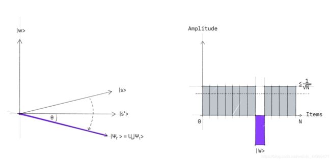
Geometrically this corresponds to a reflection of the state $|s⟩$ about $|s^{\prime }⟩$. This transformation means that the amplitude in front of the $|w⟩$ state becomes negative, which in turn means that the average amplitude (indicated by a dashed line) has been lowered.

Step 3: We now apply an additional reflection $(U_s)$ about the state $|s⟩:U_s=2|s⟩⟨s|-1$. This transformation maps the state to $U_s{U}_f|s⟩$ and completes the transformation.

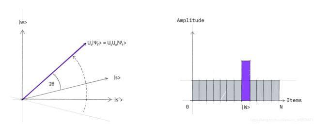
Two reflections always correspond to a rotation. The transformation $U_s{U}_f$ rotates the initial state $|s⟩$ closer towards the winner $|w⟩$. The action of the reflection $U_s$ in the amplitude bar diagram can be understood as a reflection about the average amplitude. Since the average amplitude has been lowered by the first reflection, this transformation boosts the negative amplitude of $|w⟩$ to roughly three times its original value, while it decreases the other amplitudes. We then go to step 2 to repeat the application. This procedure will be repeated several times to zero in on the winner.

After t steps we will be in the state $|{\psi }_t⟩$ where: $|{\psi }_t⟩=(U_s{U}_f{)}^t|s⟩$.

How many times do we need to apply the rotation? It turns out that roughly \sqrt{N} rotations suffice. This becomes clear when looking at the amplitudes of the state $|\psi ⟩$. We can see that the amplitude of $|w⟩$ grows linearly with the number of applications $\sim t{N}^{-1/2}$. However, since we are dealing with amplitudes and not probabilities, the vector space’s dimension enters as a square root. Therefore it is the amplitude, and not just the probability, that is being amplified in this procedure.

In the case that there are multiple solutions, M, it can be shown that roughly $\sqrt{(N/M)}$ rotations will suffice.