【机器学习与算法】python手写算法：xgboost源码复现

背景知识

关于XGB原理的解释与推导，最好就直接参看原作者陈天奇大神的PPT，这里对原理不再赘述，直接附上链接：
tqchen/pdf/BoostedTree.pdf.
根据PPT的内容，我们来用python对XGB算法进行一个复现，实现两种目标函数的拟合：linear和logistic，这两种目标函数的公式如下：

当用python复现一遍xgboost算法后，相信一定会对算法过程、每个参数的含义及作用节点、作用效果有一个更清晰的认识。

上代码

import pandas as pd
import numpy as np

class XGB:
    
    def __init__(self, 
                 base_score = 0.5,
                 max_depth=3,
                 n_estimators=10,
                 learning_rate = 0.1,
                 reg_lambda = 1,
                 gamma = 0,
                 min_child_sample = None,
                 min_child_weight = 1,
                 objective = 'linear'):
        
        self.base_score = base_score  #最开始时给叶子节点权重所赋的值，默认0.5，迭代次数够多的话，结果对这个初值不敏感
        self.max_depth = max_depth  #最大数深度
        self.n_estimators = n_estimators  #树的个数
        self.learning_rate = learning_rate  #学习率，别和梯度下降里的学习率搞混了，这里是每棵树要乘以的权重系数
        self.reg_lambda = reg_lambda  #L2正则项的权重系数
        self.gamma = gamma  #正则项中，叶子节点数T的权重系数
        self.min_child_sample = min_child_sample #每个叶子节点的样本数（自己加的）
        self.min_child_weight = min_child_weight #每个叶子节点的Hessian矩阵和，下面代码会细讲
        self.objective = objective #目标函数，可选linear和logistic
        self.tree_structure = {} #用一个字典来存储每一颗树的树结构
        

    def xgb_cart_tree(self, X, w, m_dpth):
        '''
        递归的方式构造XGB中的Cart树
        X：训练数据集
        w：每个样本的权重值，递归赋值
        m_dpth：树的深度
        '''
        
        #边界条件：递归到指定最大深度后，跳出
        if m_dpth > self.max_depth:
            return
        
        best_var, best_cut = None, None
        #这里增益的初值一定要设置为0，相当于对树做剪枝，即如果算出的增益小于0则不做分裂
        max_gain = 0
        G_left_best, G_right_best, H_left_best, H_right_best = 0,0,0,0
        #遍历每个变量的每个切点，寻找分裂增益gain最大的切点并记录下来
        for item in [x for x in X.columns if x not in ['g','h','y']]:
            for cut in list(set(X[item])):
                
                #这里如果指定了min_child_sample则限制分裂后叶子节点的样本数都不能小于指定值
                if self.min_child_sample:
                    if (X.loc[X[item]<cut].shape[0]<self.min_child_sample)\
                        |(X.loc[X[item]>=cut].shape[0]<self.min_child_sample):
                        continue
                
                G_left = X.loc[X[item]<cut,'g'].sum()
                G_right = X.loc[X[item]>=cut,'g'].sum()
                H_left = X.loc[X[item]<cut,'h'].sum()
                H_right = X.loc[X[item]>=cut,'h'].sum()
                
                #min_child_weight在这里起作用，指的是每个叶子节点上的H，即目标函数二阶导的加和
                #当目标函数为linear，即1/2*(y-y_hat)**2时，它的二阶导是1，那min_child_weight就等价于min_child_sample
                #当目标函数为logistic，其二阶导为sigmoid(y_hat)*(1-sigmoid(y_hat))，可理解为叶子节点的纯度，更详尽的解释可参看：
                #https://stats.stackexchange.com/questions/317073/explanation-of-min-child-weight-in-xgboost-algorithm#
                if self.min_child_weight:
                    if (H_left<self.min_child_weight)|(H_right<self.min_child_weight):
                        continue
                
                gain = G_left**2/(H_left + self.reg_lambda) + \
                       G_right**2/(H_right + self.reg_lambda) - \
                       (G_left + G_right)**2/(H_left + H_right + self.reg_lambda)
                gain = gain/2 - self.gamma
                if gain > max_gain:
                    best_var, best_cut = item, cut
                    max_gain = gain
                    G_left_best, G_right_best, H_left_best, H_right_best = G_left, G_right, H_left, H_right
        
        #如果遍历完找不到可分列的点，则返回None
        if best_var is None:
            return None
        
        #给每个叶子节点上的样本分别赋上相应的权重值
        id_left = X.loc[X[best_var]<best_cut].index.tolist()
        w_left = - G_left_best / (H_left_best + self.reg_lambda)

        id_right = X.loc[X[best_var]>=best_cut].index.tolist()
        w_right = - G_right_best / (H_right_best + self.reg_lambda)
        
        w[id_left] = w_left
        w[id_right] = w_right
        
        #用俄罗斯套娃式的json串把树的结构给存下来
        tree_structure = {(best_var,best_cut):{}}
        tree_structure[(best_var,best_cut)][('left',w_left)] = self.xgb_cart_tree(X.loc[id_left], w, m_dpth+1)
        tree_structure[(best_var,best_cut)][('right',w_right)] = self.xgb_cart_tree(X.loc[id_right], w, m_dpth+1)
                
        return tree_structure

    
    def _grad(self, y_hat, Y):
        '''
        计算目标函数的一阶导
        支持linear和logistic
        '''

        if self.objective == 'logistic':
            y_hat = 1.0/(1.0+np.exp(-y_hat))
            return y_hat - Y
        elif self.objective == 'linear':
            return y_hat - Y
        else:
            raise KeyError('objective must be linear or logistic!')
    

    def _hess(self,y_hat, Y):
        '''
        计算目标函数的二阶导
        支持linear和logistic
        '''
        
        if self.objective == 'logistic':
            y_hat = 1.0/(1.0+np.exp(-y_hat))
            return y_hat * (1.0 - y_hat)
        elif self.objective == 'linear':
            return np.array([1]*Y.shape[0])
        else:
            raise KeyError('objective must be linear or logistic!')
            
    
    def fit(self, X:pd.DataFrame, Y):
        '''
        根据训练数据集X和Y训练出树结构和权重
        '''
        
        if X.shape[0]!=Y.shape[0]:
            raise ValueError('X and Y must have the same length!')
            
        X = X.reset_index(drop='True')
        Y = Y.values
        #这里根据base_score参数设定权重初始值
        y_hat = np.array([self.base_score]*Y.shape[0])
        for t in range(self.n_estimators):
            
            print('fitting tree {}...'.format(t+1))

            X['g'] = self._grad(y_hat, Y)
            X['h'] = self._hess(y_hat, Y)
            
            f_t = pd.Series([0]*Y.shape[0])
            self.tree_structure[t+1] = self.xgb_cart_tree(X, f_t, 1)

            y_hat = y_hat + self.learning_rate * f_t

            print('tree {} fit done!'.format(t+1))
            
        print(self.tree_structure)
            
        
    def _get_tree_node_w(self, X, tree, w):
        '''
        以递归的方法，把树结构解构出来，把权重值赋到w上面
        '''

        if not tree is None:
            k = list(tree.keys())[0]
            var,cut = k[0],k[1]
            X_left = X.loc[X[var]<cut]
            id_left = X_left.index.tolist()
            X_right = X.loc[X[var]>=cut]
            id_right = X_right.index.tolist()
            for kk in tree[k].keys():
                if kk[0] == 'left':
                    tree_left = tree[k][kk]
                    w[id_left] = kk[1]
                elif kk[0] == 'right':
                    tree_right = tree[k][kk]
                    w[id_right] = kk[1]
        
            self._get_tree_node_w(X_left, tree_left, w)
            self._get_tree_node_w(X_right, tree_right, w)
            
        
    def predict_raw(self, X:pd.DataFrame):
        '''
        根据训练结果预测
        返回原始预测值
        '''
        
        X = X.reset_index(drop='True')
        Y = pd.Series([self.base_score]*X.shape[0])

        for t in range(self.n_estimators):
            tree = self.tree_structure[t+1]
            y_t = pd.Series([0]*X.shape[0])
            self._get_tree_node_w(X, tree, y_t)
            Y = Y + self.learning_rate * y_t
            
        return Y
    
    
    def predict_prob(self, X:pd.DataFrame):
        '''
        当指定objective为logistic时，输出概率要做一个logistic转换
        '''
        
        Y = self.predict_raw(X)
        sigmoid = lambda x:1/(1+np.exp(-x))
        Y = Y.apply(sigmoid)
        
        return Y

结果对比

1、目标函数：linear

目标函数：1/2 *（y_hat - y） ** 2
一阶导数（grad）：y_hat - y
二阶导数（hess）：1

#INPUT
X = df[[x for x in df.columns if x!='y']]
Y = df['y']
xgb = XGB(n_estimators=2, max_depth=2, reg_lambda=1, min_child_weight=1, objective='linear')
xgb.fit(X,Y)

#OUTPUT：
fitting tree 1...
tree 1 fit done!
fitting tree 2...
tree 2 fit done!
{1: {('V2', 0.166474): {('left', -0.46125265392781317): {('V4', 0.30840057): {('left', -0.4622741764080765): None, ('right', 0.25): None}}, ('right', -0.32500000000000001): {('V3', 0.07025362056365991): {('left', -0.36363636363636365): None, ('right', 0.083333333333333329): None}}}}, 2: {('V2', 0.166474): {('left', -0.41514992294866337): {('V4', 0.30840057): {('left', -0.41609588460960778): None, ('right', 0.23749999999999999): None}}, ('right', -0.29296717171717179): {('V3', 0.07025362056365991): {('left', -0.32793388429752085): None, ('right', 0.076388888888888909): None}}}}}

这里我们指定训练一个两棵树，每棵树深度为2的XGBooster，L2正则项系数指定为1，min_child_weight指定为1，其它用默认参数。
OUTPUT中以json串的形式输出了这两颗树的结构及叶子权重，不太方便看，我们把第一课树重画成树结构，如下图：

接下来我们来调用一下xgboost包，在同样的数据集上，设定同样的参数，来训练一下，并通过自带的plot_tree函数画出它的第一棵树来对比一下：

from xgboost import XGBClassifier as xx
clf = xx(n_estimators=2, max_depth=2, objective = 'reg:linear',min_child_weight=1, learning_rate=0.1)
clf.fit(X,Y)

from xgboost import plot_tree
import matplotlib.pyplot as plt
import os
os.environ["PATH"] += os.pathsep + 'D:/Program Files/graphviz/bin/'
plot_tree(clf, num_trees=0)
fig = plt.gcf()
fig.set_size_inches(100, 50)
plt.show()

嗯，一个是分裂点有点有点差异，这是因为我们的程序里直接选取了变量里面的原值作为分裂点；而xgboost包里计算了相邻两个值的中间值，但分出来的样本数量是一样的；二是每个叶子节点的权重都小了10倍，这是因为xgboost画树的时候，把learning_rate也给乘上去了，我们设定的learning_rate就是0.1。
再来对比一下predict的结果：

#python代码结果
#INPUT：
xgb.predict_raw(X).head()
#OUTUT：
0    0.412163
1    0.412163
2    0.412163
3    0.412163
4    0.412163
dtype: float64

#xgboost包结果：
#INPUT:
y_p2 = clf.predict_proba(X)
y_p2[:5]
#OUTPUT：
array([[ 0.58783698,  0.41216299],
       [ 0.58783698,  0.41216299],
       [ 0.58783698,  0.41216299],
       [ 0.58783698,  0.41216299],
       [ 0.58783698,  0.41216299]], dtype=float32)

嗯，也是一样的。

2、目标函数：logistic

目标函数：y * ln(1 + exp(-y_hat)) + (1 - y) * ln(1+exp(y_hat))
一阶导数（grad）：sigmoid(y_hat) - y
二阶导数（hess）：sigmoid(y_hat) * (1 - sigmoid(y_hat))
只需要把obeject参数更改为’logistic’就可以了，这里我们只跑一棵树看下。

#INPUT:
X = df[[x for x in df.columns if x!='y']]
Y = df['y']
xgb = XGB(n_estimators=1, max_depth=2, reg_lambda=1, min_child_weight=1, objective='logistic')
xgb.fit(X,Y)

#OUTPUT:
fitting tree 1...
tree 1 fit done!
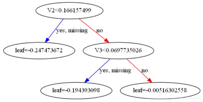
{1: {('V2', 0.166474): {('left', -2.4747364708703801): None, ('right', -1.7978275668285353): {('V3', 0.07025362056365991): {('left', -1.9439309135627878): None, ('right', -0.051630205839361273): None}}}}}

同样把树整理一下：

发现分裂节点的选取和用linear目标函数时是一样的，除了左叶子节点因为min_child_weight的原因，没有继续分裂。
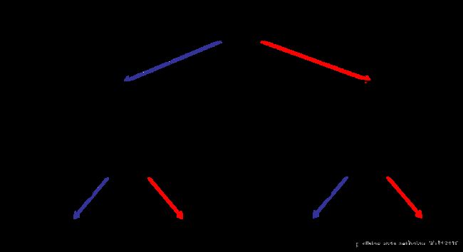
再对比一下xgboost包里跑出的树长什么样，注意这里base_score我们做了调整，默认是0.5，但是xgboost包里面第一步迭代的时候不会对这个初值先sigmoid转换，再算一阶二阶导，所以我们强行转换后再赋值到base_score里，让它和我们的代码保持一致：

clf = xx(n_estimators=1, max_depth=2, objective = 'binary:logistic',min_child_weight=1, learning_rate=0.1, base_score=1/(1+np.exp(-0.5)))
clf.fit(X,Y)

plot_tree(clf, num_trees=0)
fig = plt.gcf()
fig.set_size_inches(100, 50)
plt.show()

嗯，也是一样的树结构。
再来对比一下predict的结果，这里要注意，目标函数为logistic的时候，输出结果要做一个sigmoid转换，所以不同于上面目标函数为linear的时候调用predict_raw，这里我们需要调用predict_prob函数：

#python代码结果：
#INPUT：
xgb.predict_prob(X).head()
#OUTPUT：
0    0.562798
1    0.562798
2    0.562798
3    0.562798
4    0.562798
dtype: float64

#xgboost包结果：
#INPUT：
y_p2 = clf.predict_proba(X)
y_p2[:5]
#OUTPUT：
array([[ 0.43720174,  0.56279826],
       [ 0.43720174,  0.56279826],
       [ 0.43720174,  0.56279826],
       [ 0.43720174,  0.56279826],
       [ 0.43720174,  0.56279826]], dtype=float32)

也是一样的。

---

最后，欢迎阅读其它算法的python实现：
【机器学习与算法】python手写算法：Cart树
【机器学习与算法】python手写算法：带正则化的逻辑回归
【机器学习与算法】python手写算法：xgboost算法
【机器学习与算法】python手写算法：Kmeans和Kmeans++算法
【机器学习与算法】python手写算法：softmax回归