PyTorch深度学习实践 Lecture02 线性模型

Author ：Horizon Max

✨ 编程技巧篇：各种操作小结

机器视觉篇：会变魔术 OpenCV

深度学习篇：简单入门 PyTorch

神经网络篇：经典网络模型

算法篇：再忙也别忘了 LeetCode

视频链接：Lecture 02 Linear_Model
文档资料：

//Here is the link:
课件链接：https://pan.baidu.com/s/1vZ27gKp8Pl-qICn_p2PaSw
提取码：cxe4

Linear Modle（线性模型）

一个简单的 练习 ：

给定 3组 数据，即学习 X 小时（hours）可以得到 Y 分（points）；

X（hours）	Y（points）
1	2
2	4
3	6
预测学习 4 小时（hours）可以得到 ？ 分（points）：
X（hours）	Y（points）
--------	-----
4	？

概述

Linear Regression

根据上面的问题我们可以建立一个简单的线性模型，即 Y = W * X ；

如下图所示 ：

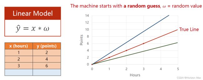
基本步骤 ：
1、根据给定的 3组 数据建立一个线性模型（即拟合一个线性函数）；
2、不断调整改变参数 W ，使尽可能多的点落在拟合的直线上（即图中的True Line）；
3、将 X=4 输入到建立的模型当中，得到预测 学习4个小时后的结果 Y-hat 分。

Loss & Cost

我们使用 Loss（损失函数）或 Cost（代价函数）来评价模型的好坏；

Cost（代价函数）= Loss（损失函数）/ 样本数（N）

在这里使用的是 均方误差 MSE（Mean Square Error），其计算公式如下：

Compute Cost

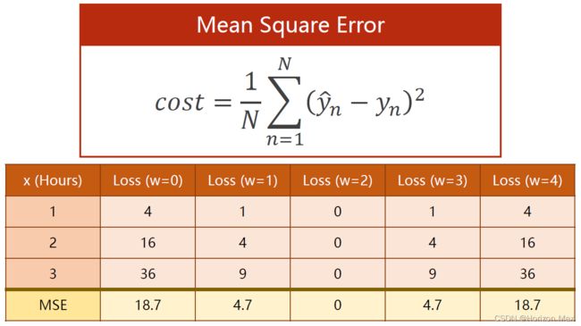
计算各参数 W 对应的 Cost 值

Code

# Here is the code :

import numpy as np
import matplotlib.pyplot as plt
 
x_data = [1.0, 2.0, 3.0]
y_data = [2.0, 4.0, 6.0]
 
def forward(x):  # 定义前向传播
    return x*w
 
def loss(x, y):  # 定义损失函数
    y_pred = forward(x)
    return (y_pred - y)**2
 
w_list = []
mse_list = []
for w in np.arange(0.0, 4.1, 0.1):  # 使用穷举法来遍历 W 值
    print("w=", w)
    l_sum = 0
    for x_val, y_val in zip(x_data, y_data):
        y_pred_val = forward(x_val)
        loss_val = loss(x_val, y_val)
        l_sum += loss_val
        print('\t', x_val, y_val, y_pred_val, loss_val)
    print('MSE=', l_sum/3)
    w_list.append(w)
    mse_list.append(l_sum/3)
    
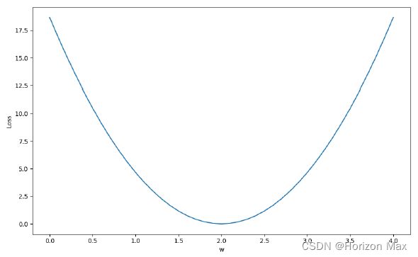
plt.plot(w_list,mse_list)
plt.ylabel('Loss')
plt.xlabel('w')
plt.show()    

运行结果

w= 0.0
1.00 2.00 0.00 4.00 
2.00 4.00 0.00 16.00
3.00 6.00 0.00 36.00
MSE= 18.666666666666668
w= 0.1
1.00 2.00 0.10 3.61
2.00 4.00 0.20 14.44 
3.00 6.00 0.30 32.49
MSE= 16.846666666666668
w=0.2
1.00 2.00 0.20 3.24 
2.00 4.00 0.40 12.96
3.00 6.00 0.60 29.16
MSE= 15.120000000000003
w= 0.30000000000000004
1.00 2.00 0.30 2.89
2.00 4.00 0.60 11.56
3.00 6.00 0.90 26.01
MSE= 13.486666666666665
w=0.4
1.00 2.00 0.40 2.56 
2.00 4.00 0.80 10.24 
3.00 6.00 1.20 23.04
MSE= 11.946666666666667
w=0.5
1.00 2.00 0.50 2.25 
2.00 4.00 1.00 9.00
3.00 6.00 1.50 20.25
MSE= 10.5

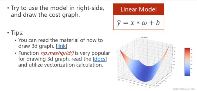
Exercise

Code

# Here is the code :

import numpy as np
import matplotlib.pyplot as plt
from mpl_toolkits.mplot3d import Axes3D    # 3D绘图

x_data = [1.0, 2.0, 3.0]
y_data = [2.0, 4.0, 6.0]

def forward(x):     # 定义前向传播
    return x * w + b

def loss(x, y):     # 定义loss函数
    y_pred = forward(x)
    return (y_pred - y) ** 2

w_list = []      # 空列表用于存放w、b、mse值
b_list = []
mse_list = []

for w in np.arange(0.0, 4.1, 0.1):      # 穷举法遍历 w [0.0 ~ 4.1)，间隔0.1
    for b in np.arange(-2.0, 2.1, 0.1):      # 穷举法遍历 b [-2.0 ~ 2.0)，间隔0.1
        l_sum = 0
        for x_val, y_val in zip(x_data, y_data):
            y_pred_val = forward(x_val)
            loss_val = loss(x_val, y_val)
            l_sum += loss_val      # 将拟合过程中得到的每个（Y-hat-Y）值累加（Loss）
        w_list.append(w)
        b_list.append(b)
        mse_list.append(l_sum/3)      # Loss值 / 样本数得到 Cost值

mse_list = np.array(mse_list)     # 转变成np.array格式便于绘图
mse_list = mse_list.reshape(41, 41)
mse_list = mse_list.transpose()

w, b = np.meshgrid(np.unique(w_list), np.unique(b_list))      # 需要转换成np.array格式
                                                              # np.meshgrid()函数自动坐标矩阵

fig = plt.figure(figsize=(8, 8))
ax = Axes3D(fig)

surf = ax.plot_surface(w, b, mse_list,
                       rstride=1,     # 行(row)的跨度
                       cstride=1,     # 列(column)的跨度
                       cmap=plt.get_cmap('rainbow'))

ax.set_zlim(0, 40)     # Z轴lim
ax.set_xlabel('W')     # 设置角标
ax.set_ylabel('b')
plt.title("Cost Values")
fig.colorbar(surf, shrink=0.5, aspect=10)  # shrink:色彩条与图形高度的比例, aspect:色彩条本身的长宽比

plt.show()

运行结果

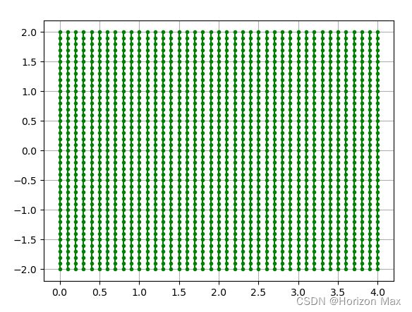
np.meshgrid()函数

w, b = np.meshgrid(np.unique(w_list), np.unique(b_list))      # 需要转换成np.array格式
                                                              # np.meshgrid()函数自动坐标矩阵
print('w = ', w)
print('b = ', b)

plt.plot(w, b,
         color='g',         # 设置颜色为green
         marker='.',        # 设置点类型为圆点
         linestyle='-')      # 点与点之间用-连接
plt.grid(True)
plt.show()

w = [[0.  0.1 0.2 ... 3.8 3.9 4. ]
	 [0.  0.1 0.2 ... 3.8 3.9 4. ]
	 [0.  0.1 0.2 ... 3.8 3.9 4. ]
	 ...
	 [0.  0.1 0.2 ... 3.8 3.9 4. ]
	 [0.  0.1 0.2 ... 3.8 3.9 4. ]
	 [0.  0.1 0.2 ... 3.8 3.9 4. ]]


b = [[-2.  -2.  -2.  ... -2.  -2.  -2. ]
	 [-1.9 -1.9 -1.9 ... -1.9 -1.9 -1.9]
	 [-1.8 -1.8 -1.8 ... -1.8 -1.8 -1.8]
	 ...
	 [ 1.8  1.8  1.8 ...  1.8  1.8  1.8]
	 [ 1.9  1.9  1.9 ...  1.9  1.9  1.9]
	 [ 2.   2.   2.  ...  2.   2.   2. ]]

每一个点的坐标为 （w，b）

附录：相关文档资料

PyTorch 官方文档： PyTorch Documentation
PyTorch 中文手册： PyTorch Handbook

《PyTorch深度学习实践》系列链接：

  Lecture01 Overview
  Lecture02 Linear_Model
  Lecture03 Gradient_Descent
  Lecture04 Back_Propagation
  Lecture05 Linear_Regression_with_PyTorch
  Lecture06 Logistic_Regression
  Lecture07 Multiple_Dimension_Input
  Lecture08 Dataset_and_Dataloader
  Lecture09 Softmax_Classifier
  Lecture10 Basic_CNN
  Lecture11 Advanced_CNN
  Lecture12 Basic_RNN
  Lecture13 RNN_Classifier