R语言数据分析、展现与实例(02)
R语言数据分析、展现与实例(02)
数据输入
> mydata <- data.frame(age=numeric(0),gender=character(0),weight=numeric(0)) #创建空数据框
> mydata <- edit(mydata) #打开编辑框进行编辑,并将结果赋值给原数据框 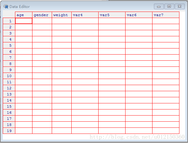
输入数据,直接退出即可保存
> mydata
  age gender weight
1   1      g      3
2   2      b      3
3   3      b      3
> mydata <- edit(mydata)    #直接打开编辑框也可进行变量的添加,在var双击即可
> fix(mydata)      #打开编辑框进行编辑,可直接保存到原文件
> mydata
  age gender weight
1   1      G      3
2   2      b      3
3   3      b      3
>
读文本文件数据
- 先设置工作目录,把文本文件放到该目录下
> (x=read.table("abc.txt"))
   V1     V2     V3
1 age gender weight
2   1      G      3
3   2      b      3
4 3 b 3- 直接读取其他目录的文本文件
> abc <- read.table("D:/R_workspace/Dataguru/week2/abc.txt",header=T)
> abc
  age gender weight
1   1      G      3
2   2      b      3
3   3      b      3
在Rstudio中读取
在import dataset 中文本或excel的数据均可通过剪贴板操作
> y<-read.table("clipboard",header = F)   #不读列头
> y
   V1     V2     V3
1 age gender weight
2   1      G      3
3   2      b      3
4   3      b      3
> y<-read.table("clipboard",header = T)  # 读列头
> y
  age gender weight
1   1      G      3
2   2      b      3
3 3 b 3- 读excel文件数据
方法1:先把excel另存为空格分隔的prn文本格式再读
> w<- read.table("tt.prn",header = F)
> w
    V1   V2
1 商品 价格
2   12   21
方法2:安装RODBC包,再通过ODBC读

> library(RODBC)
> Z<- odbcConnectExcel("tt.xls")
> (w<-sqlFetch(Z,"Sheet1"))
  商品 价格
1   12   21
2   22   23
3   NA   NA
4   21   22
>
mistake:
> library(RODBC)
> Z<- odbcConnectExcel("tt.xls")
Error in odbcConnectExcel("tt.xls") :
  odbcConnectExcel is only usable with 32-bit Windows
换成32bit的R运行即可
- 导入XML数据
XML包
安装XML包
> library(XML)
>  fileName<-system.file("exampleData","include.xml",package="XML")
> fileName
[1] "D:/R_library/XML/exampleData/include.xml"
> root<-xmlParse(fileName)            #用xmlParse读取文件
> root

<doc xmlns:xi="http://www.w3.org/2001/XInclude">
  <caveat>
    <para>This is a caveat that we repeat often.para>
  caveat>
  <section>
    <title>Atitle>

    <caveat>
      <para>This is a caveat that we repeat often.para>
    caveat>

  section>
  <section>
    <title>Btitle>

    <caveat>
      <para>This is a caveat that we repeat often.para>
    caveat>

  section>
doc>
读取SAS、SPSS、Stata文件
foreign包
- spss文件 read.spss()
- SAS文件 read.xport()
- Stata文件 read.dta()
- Hmisc包
- SPSS文件 spss.get()
连接数据库
- RODBC包
> library(RODBC)
> conn <- odbcConnectAccess2007(access.file = "D:/R_workspace/Dataguru/week2/Stock.accdb",uid = "test",pwd = "test")
> ZGSH <- sqlQuery(conn,"SELECT Stkcd,Trddt,Opnprc,Hiprc,Loprc,Clsprc,Adjprcwd,Dretwd FROM Stock WHERE Stkcd = 600028")
> View(ZGSH)
> ZGSH
  ………………
> stk.query <- "SELECT Stock.Stkcd , Stock.Trddt , Stock.Adjprcwd , Stock.Dsmvosd FROM Stock INNER JOIN Company ON Stock.Stkcd = Company.Stkcd WHERE Company.Listdt <= #1/1/2009#"
> data.list.09 <- sqlQuery(conn , stk.query)
> View(data.list.09)
> View(data.list.09)
> close(conn)            #关闭数据库连接
- RODBC包
mistake:
在RStudio中,若R包安装成功但无法加载,将安装library目录下的与R包同名的文件夹删除,再重新安装R包即可。
写数据文件
- write()函数 #主要保存矩阵和向量
- write.table()函数
- write. csv()函数
数据整理
- 了解当前数据状态
- head()与tail() # 查看数据前六行 后六行
- length()、dim()、ncol()、nrow()
- str()与ls()
- 选取数据子集
- 数据合并
- 数据的编辑
其他
了解当前
> head(ZGSH)
   Stkcd      Trddt Opnprc Hiprc Loprc Clsprc Adjprcwd    Dretwd
1 600028 2009-01-05   7.10  7.21  7.06   7.19 10.70134  0.024217
2 600028 2009-01-06   7.15  7.44  7.12   7.41 11.02878  0.030598
3 600028 2009-01-07   7.40  7.42  7.25   7.25 10.79064 -0.021592
4 600028 2009-01-08   7.14  7.16  6.96   7.14 10.62692 -0.015172
5 600028 2009-01-09   7.08  7.16  7.06   7.14 10.62692  0.000000
6 600028 2009-01-12   7.09  7.17  7.02   7.09 10.55251 -0.007003
> tail(ZGSH)
      Stkcd      Trddt Opnprc Hiprc Loprc Clsprc Adjprcwd    Dretwd
1199 600028 2013-12-24   4.62  4.64  4.52   4.57 10.43269 -0.008677
1200 600028 2013-12-25   4.57  4.61  4.54   4.58 10.45552  0.002188
1201 600028 2013-12-26   4.59  4.59  4.42   4.48 10.22724 -0.021834
1202 600028 2013-12-27   4.48  4.52  4.41   4.48 10.22724  0.000000
1203 600028 2013-12-30   4.50  4.51  4.42   4.43 10.11309 -0.011161
1204 600028 2013-12-31   4.41  4.50  4.41   4.48 10.22724  0.011287
> head(ZGSH,3)
   Stkcd      Trddt Opnprc Hiprc Loprc Clsprc Adjprcwd    Dretwd
1 600028 2009-01-05   7.10  7.21  7.06   7.19 10.70134  0.024217
2 600028 2009-01-06   7.15  7.44  7.12   7.41 11.02878  0.030598
3 600028 2009-01-07   7.40  7.42  7.25   7.25 10.79064 -0.021592
> length(c(1,2,3,4,5))     #查看数据长度
[1] 5
> dim(ZGSH)  #查看多维数据大小
[1] 1204    8
> nrow(ZGSH)
[1] 1204
> ncol(ZGSH)
[1] 8
> str(ZGSH)           #查看数据类型等
'data.frame':   1204 obs. of  8 variables:
 $ Stkcd   : int  600028 600028 600028 600028 600028 600028 600028 600028 600028 600028 ...
 $ Trddt   : Factor w/ 1204 levels "2009-01-05","2009-01-06",..: 1 2 3 4 5 6 7 8 9 10 ...
 $ Opnprc  : num  7.1 7.15 7.4 7.14 7.08 7.09 7.03 7.05 7.15 7.21 ...
 $ Hiprc   : num  7.21 7.44 7.42 7.16 7.16 7.17 7.11 7.25 7.25 7.59 ...
 $ Loprc   : num  7.06 7.12 7.25 6.96 7.06 7.02 6.97 7.02 7.11 7.21 ...
 $ Clsprc  : num  7.19 7.41 7.25 7.14 7.14 7.09 7.06 7.24 7.17 7.43 ...
 $ Adjprcwd: num  10.7 11 10.8 10.6 10.6 ...
 $ Dretwd  : num  0.0242 0.0306 -0.0216 -0.0152 0 ...
> ls(ZGSH)   #查看变量
[1] "Adjprcwd" "Clsprc"   "Dretwd"   "Hiprc"    "Loprc"    "Opnprc"   "Stkcd"    "Trddt"
选取数据子集
> y <- c(1,8,4,7,6,0,4)
> y[c(1,3)]
[1] 1 4
> y[2:4]
[1] 8 4 7
> x <- subset(y,y>3)     # 选取y中y>3的子集
> x
[1] 8 4 7 6 4
> which(y>3)       #返回y中y>3的元素的位置
[1] 2 3 4 5 7
> y[which(y>3)]
[1] 8 4 7 6 4
> a <- c(1,3,5)
> a[-2]        #去掉a中第二个元素
[1] 1 5
> x <- matrix (1:10, nrow = 2)
> x
     [,1] [,2] [,3] [,4] [,5]
[1,]    1    3    5    7    9
[2,]    2    4    6    8   10
> x[,2]      #选取第二列
[1] 3 4
> x[1,c(4,5)]      #选取第一行第四列和第五列
[1] 7 9

数据框形式的选取
> x <- data.frame(x)    #将x转换成数据框的形式
> x
  X1 X2 X3 X4 X5
1  1  3  5  7  9
2  2  4  6  8 10
> x[,1]
[1] 1 2
> x[1]
  X1
1  1
2  2
> x$X1        #  "$"这个符号相当于“的”
[1] 1 2

# 列表的选取
> g <- "I am happy"
> h <- c(1,2,3,4)
> j <- matrix(1:9,nrow =3)
> k <- c("good","excellent","poor")
> mylist <- list(g,h,j,k)
> mylist
[[1]]
[1] "I am happy"

[[2]]
[1] 1 2 3 4

[[3]]
     [,1] [,2] [,3]
[1,]    1    4    7
[2,]    2    5    8
[3,]    3    6    9

[[4]]
[1] "good"      "excellent" "poor"

> mylist[3]           #用一个中括号选取出来还是一个list
[[1]]
     [,1] [,2] [,3]
[1,]    1    4    7
[2,]    2    5    8
[3,]    3    6    9

> mylist[[3]]      # 用两个中括号选取处理啊就是数据原本的格式
     [,1] [,2] [,3]
[1,]    1    4    7
[2,]    2    5    8
[3,]    3    6    9
数据的合并
> x <- 1:3
> y <- c(3,4,5)
> c(x,y)               #向量的合并
[1] 1 2 3 3 4 5

#矩阵合并
> cbind(1,1:4)     #按行合并
     [,1] [,2]
[1,]    1    1
[2,]    1    2
[3,]    1    3
[4,]    1    4
> rbind(1:2,1:6)      #按列合并
     [,1] [,2] [,3] [,4] [,5] [,6]
[1,]    1    2    1    2    1    2
[2,]    1    2    3    4    5    6


#数据框的合并
> authors <- data.frame(
+     surname = I(c("Tukey", "Venables", "Tierney", "Ripley", "McNeil")),
+     nationality = c("US", "Australia", "US", "UK", "Australia"),
+     deceased = c("yes", rep("no", 4)) )
> authors
   surname nationality deceased
1    Tukey          US      yes
2 Venables   Australia       no
3  Tierney          US       no
4   Ripley          UK       no
5   McNeil   Australia       no
> books <- data.frame(
+     name = I(c("Tukey", "Venables", "Tierney",
+                "Ripley", "Ripley", "McNeil", "R Core")),
+     title = c("Exploratory Data Analysis",
+               "Modern Applied Statistics ...",
+               "LISP -STAT",
+               "Spatial Statistics", "Stochastic Simulation",
+               "Interactive Data Analysis",
+               "An Introduction to R"),
+     other.author = c(NA, "Ripley", NA, NA, NA, NA,
+                      "Venables & Smith"))
> books
      name                         title     other.author
1    Tukey     Exploratory Data Analysis             <NA>
2 Venables Modern Applied Statistics ...           Ripley
3  Tierney                    LISP -STAT             <NA>
4   Ripley            Spatial Statistics             <NA>
5   Ripley         Stochastic Simulation             <NA>
6   McNeil     Interactive Data Analysis             <NA>
7   R Core          An Introduction to R Venables & Smith
> merge(authors,books,by.x = "surname", by.y ="name",all = TRUE)
   surname nationality deceased                         title
1   McNeil   Australia       no     Interactive Data Analysis
2   R Core        <NA>     <NA>          An Introduction to R
3   Ripley          UK       no            Spatial Statistics
4   Ripley          UK       no         Stochastic Simulation
5  Tierney          US       no                    LISP -STAT
6    Tukey          US      yes     Exploratory Data Analysis
7 Venables   Australia       no Modern Applied Statistics ...
      other.author
1             <NA>
2 Venables & Smith
3             <NA>
4             <NA>
5             <NA>
6             <NA>
7           Ripley
> paste("A",1:6,sep = "")      #连接A和1:6 中间不加字符
[1] "A1" "A2" "A3" "A4" "A5" "A6"
> paste("A",1:6,sep = "@")      #连接A和1:6,中间以@连接
[1] "A@1" "A@2" "A@3" "A@4" "A@5" "A@6"
删除对象列表
> aa <-1:4
> aa
[1] 1 2 3 4
> rm(aa)
> aa
Error: object 'aa' not found
删除缺失值
> omit <- read.csv("D:/R_workspace/Dataguru/week2/omit.csv",header = T)
> omit
  cd   Trddit Opnprc Hipri
1  1     <NA>     12   5.5
2  1 2009/1/3     21    NA
3  1 2009/1/2     12   2.3
4  1 2009/2/3     32   2.3
5  1 2009/2/3     43   2.1
6  1 2009/1/2    543   9.1
> omit1 <- na.omit(omit)        #删除omit文件中的缺失值,并将处理后的文件存入omit1
> omit1
  cd   Trddit Opnprc Hipri
3  1 2009/1/2     12   2.3
4  1 2009/2/3     32   2.3
5  1 2009/2/3     43   2.1
6 1 2009/1/2 543 9.1- tansfrom函数 #用于变换数据中的对象
> stock <- read.csv("D:/R_workspace/Dataguru/week2/price.csv",header = T)
> stock
   No Stkcd     Trddt Opnprc Hiprc Loprc Clsprc
1   1     1  2009/1/5   9.57  9.74  9.51   9.71
2   2     1  2009/1/6   9.80 10.43  9.73  10.30
3   3     1  2009/1/7  10.20 10.40  9.99   9.99
4   4     1  2009/1/8   9.75  9.76  9.50   9.60
5   5     1  2009/1/9   9.60  9.93  9.60   9.85
6   6     1 2009/1/12   9.78 10.08  9.67   9.86
7   7     1 2009/1/13   8.88  9.63  8.88   9.47
8   8     1 2009/1/14   9.30 10.25  9.30  10.20
9   9     1 2009/1/15  10.01 10.60  9.97  10.30
10 10     1 2009/1/16  10.34 10.94 10.34  10.62
11 11     1 2009/1/19  10.65 11.35 10.65  11.11
12 12     1 2009/1/20  11.07 11.40 11.02  11.36
13 13     1 2009/1/21  11.15 12.20 11.00  11.79
14 14     1 2009/1/22  11.80 12.00 11.40  11.79
15 15     1 2009/1/23  11.58 11.93 11.58  11.64
16 16     1  2009/2/2  11.76 11.99 11.51  11.66
17 17     1  2009/2/3  11.66 12.06 11.60  11.95
18 18     1  2009/2/4  12.02 13.15 12.02  13.04
19 19     1  2009/2/5  13.07 13.20 12.63  12.80
20 20     1  2009/2/6  12.82 13.44 12.82  13.19
> transform(stock,Opnprc = -Opnprc,difference =Hiprc - Loprc)
   No Stkcd     Trddt Opnprc Hiprc Loprc Clsprc difference
1   1     1  2009/1/5  -9.57  9.74  9.51   9.71       0.23
2   2     1  2009/1/6  -9.80 10.43  9.73  10.30       0.70
3   3     1  2009/1/7 -10.20 10.40  9.99   9.99       0.41
4   4     1  2009/1/8  -9.75  9.76  9.50   9.60       0.26
5   5     1  2009/1/9  -9.60  9.93  9.60   9.85       0.33
6   6     1 2009/1/12  -9.78 10.08  9.67   9.86       0.41
7   7     1 2009/1/13  -8.88  9.63  8.88   9.47       0.75
8   8     1 2009/1/14  -9.30 10.25  9.30  10.20       0.95
9   9     1 2009/1/15 -10.01 10.60  9.97  10.30       0.63
10 10     1 2009/1/16 -10.34 10.94 10.34  10.62       0.60
11 11     1 2009/1/19 -10.65 11.35 10.65  11.11       0.70
12 12     1 2009/1/20 -11.07 11.40 11.02  11.36       0.38
13 13     1 2009/1/21 -11.15 12.20 11.00  11.79       1.20
14 14     1 2009/1/22 -11.80 12.00 11.40  11.79       0.60
15 15     1 2009/1/23 -11.58 11.93 11.58  11.64       0.35
16 16     1  2009/2/2 -11.76 11.99 11.51  11.66       0.48
17 17     1  2009/2/3 -11.66 12.06 11.60  11.95       0.46
18 18     1  2009/2/4 -12.02 13.15 12.02  13.04       1.13
19 19     1  2009/2/5 -13.07 13.20 12.63  12.80       0.57
20 20     1  2009/2/6 -12.82 13.44 12.82  13.19       0.62
names()函数 #查看或更改数据表中行和列的名字
> names(ZGSH)         #获取ZGSH的名字
[1] "Stkcd"    "Trddt"    "Opnprc"   "Hiprc"    "Loprc"
[6] "Clsprc"   "Adjprcwd" "Dretwd"
> data = (ZGSH)
> names(data) <- LETTERS[1:8]        #将字母中第1:8个字母替换原列名
> names(data)
[1] "A" "B" "C" "D" "E" "F" "G" "H"
排序
> x <-c(1,6,2,8,5)
> sort(x)        #正常对原数据进行排序
[1] 1 2 5 6 8
> order(x)    #返回排序后,原数据的位置 eg:第二个3是排在第二位的数据原来的位置是排在第三位
[1] 1 3 5 2 4
> rank(x)     #返回数据排序后的位置
[1] 1 4 2 5 3

#矩阵元素排序
> a <- matrix( c(5, 3, 4, 2, 2, 6, 8, 9, 7, 6, 12, 10, 11, 14, 13), 5)
> a
     [,1] [,2] [,3]
[1,]    5    6   12
[2,]    3    8   10
[3,]    4    9   11
[4,]    2    7   14
[5,]    2    6   13
> a[order(a[,1]),]              #按矩阵第一列进行排序
     [,1] [,2] [,3]
[1,]    2    7   14
[2,]    2    6   13
[3,]    3    8   10
[4,]    4    9   11
[5,]    5    6   12
> a[order(a[,1],a[,2]),]     #按矩阵第一列和第二列进行排序
     [,1] [,2] [,3]
[1,]    2    6   13
[2,]    2    7   14
[3,]    3    8   10
[4,]    4    9   11
[5,]    5    6   12
> a[order(a[,1],-a[,2]),]     # 按矩阵第一列进行排序,不按第二列进行排序
     [,1] [,2] [,3]
[1,]    2    7   14
[2,]    2    6   13
[3,]    3    8   10
[4,]    4    9   11
[5,]    5    6   12
table()函数 #快速生成列联表
> ff <- factor( c("Male", "Female", "Male", "Female", "Female") )
> table(ff)     #统计ff中两类数据的个数
ff
Female   Male
     3      2
数学运算
- 算数运算符

- 逻辑运算符

> a <-c(1,2,3)
> b <-c(2,1,4)
> x <- a<=b
> x
[1] TRUE FALSE TRUE
> y <- a >= b
> y
[1] FALSE TRUE FALSE
> x&y
[1] FALSE FALSE FALSE
> x&&y
[1] FALSE
> x[1]&&y[1]
[1] FALSE
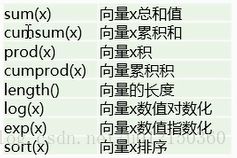
> 数学函数计算
矩阵计算

> ret <- c(0.05 ,0.09 ,0.12 , -0.10 , -0.09 ,0.01)
> arithmetic.average <- sum(ret)/length(ret)        #算术平均值
> arithmetic.average
[1] 0.01333333
> geometric.average <- prod(rep(1,length(ret))+ret)^(1/length(ret))-1
> geometric.average
[1] 0.009810423

> x<-matrix(c(1,2,3,4),nrow=2,ncol =2)
> eigen(x)             #求特征值和特征向量
$values
[1]  5.3722813 -0.3722813

$vectors
           [,1]       [,2]
[1,] -0.5657675 -0.9093767
[2,] -0.8245648  0.4159736

> det(x)    #求行列式的值
[1] -2
> rank(x)   #求矩阵的秩
[1] 1 2 3 4
> rev(x)          #求矩阵的逆
[1] 4 3 2 1
数据可视化的重要性(作图)
延伸第一节最后的综合性例子,以下是第一节例子数据框的生成
> num = seq(1078001,10378100)
> num
   [1] 1078001 1078002 1078003 1078004 1078005 1078006 1078007
   [8] 1078008 1078009 1078010 1078011 1078012 1078013 1078014
  [15] 1078015 1078016 1078017 1078018 1078019 1078020 1078021
  [22] 1078022 1078023 1078024 1078025 1078026 1078027 1078028
  [29] 1078029 1078030 1078031 1078032 1078033 1078034 1078035
  [36] 1078036 1078037 1078038 1078039 1078040 1078041 1078042
  [43] 1078043 1078044 1078045 1078046 1078047 1078048 1078049
  [50] 1078050 1078051 1078052 1078053 1078054 1078055 1078056
  [57] 1078057 1078058 1078059 1078060 1078061 1078062 1078063
  [64] 1078064 1078065 1078066 1078067 1078068 1078069 1078070
  [71] 1078071 1078072 1078073 1078074 1078075 1078076 1078077

   ……………………………………

 [967] 1078967 1078968 1078969 1078970 1078971 1078972 1078973
 [974] 1078974 1078975 1078976 1078977 1078978 1078979 1078980
 [981] 1078981 1078982 1078983 1078984 1078985 1078986 1078987
 [988] 1078988 1078989 1078990 1078991 1078992 1078993 1078994
 [995] 1078995 1078996 1078997 1078998 1078999 1079000
 [ reached getOption("max.print") -- omitted 9299100 entries ]

> x1 = round(runif(100,min=80,max=100))
> x1
  [1]  97  83  90  90  81  92  89  83 100  88  98  95  90  91  92  97  82  81  90  92  85  95  89  80
 [25]  93  99  81  97  99  86  82  92  90  85  98  86  87  93  86  97 100  94  87  93  83  83  99  93
 [49]  92  84  89  90  84 100  88  95  94  82  84  89  85  90  93  94  85  87  87  86  88  95  87 100
 [73]  90  91  87  87  81  86  98  97  98  98  95  88  97  94  95  93  83  95  84  95  85  89  95  88
 [97]  92  88  96  84
> x2 = round(rnorm(100,mean=80,sd=7))
> x2
  [1]  85  86  87  81  84  84  82  75  69  76  82  79  72  79  91  73  77  78  77  93  68  91  91  77
 [25]  87  76  79  73  87  80  71  93  82  84  83  83  79  75  78  87  75  72  85  71  91  69  93  67
 [49]  94  70  91  80  74  77  71  82  83  81  80  80  79  73  70  77  69  69  78  83  77  81  76  90
 [73]  77  77  77  80  80  80  80  75  78  74  89  77  90  90  85  73  74  90  72 104  84  74  97  81
 [97]  71  74  74  88
> x3 = round(rnorm(100,mean = 83,sd=18))
> x3
  [1]  76  69  93  57  69 109  87  96 112  90 117  85  87  70  37  82  75  66 102  52 112  54  92  44
 [25]  94  84  84  77 117  93  87  78  93  93  55 109  52  48  98  81  75  78  92  81  52  73 127  31
 [49] 127  56  65  62  98 101  91  83  98 110  76  95  94  50  69  62  71  40 100  75  81 101  99 109
 [73]  96  93  99  80  76  49  72 103  99  79  82  89 112  93  40  80 103  76 104  50  81  73 100  70
 [97]  66 104 106  64
> x3[which(x3>100)]=100
> x3
  [1]  76  69  93  57  69 100  87  96 100  90 100  85  87  70  37  82  75  66 100  52 100  54  92  44
 [25]  94  84  84  77 100  93  87  78  93  93  55 100  52  48  98  81  75  78  92  81  52  73 100  31
 [49] 100  56  65  62  98 100  91  83  98 100  76  95  94  50  69  62  71  40 100  75  81 100  99 100
 [73]  96  93  99  80  76  49  72 100  99  79  82  89 100  93  40  80 100  76 100  50  81  73 100  70
 [97]  66 100 100  64
> x = data.frame(num,x1,x2,x3)
> x
             num  x1  x2  x3
1        1078001  97  85  76
2        1078002  83  86  69
3        1078003  90  87  93
4        1078004  90  81  57
5        1078005  81  84  69
6        1078006  92  84 100
7        1078007  89  82  87
8        1078008  83  75  96
9        1078009 100  69 100
10       1078010  88  76  90
11       1078011  98  82 100
12       1078012  95  79  85
13       1078013  90  72  87
14       1078014  91  79  70
15       1078015  92  91  37
16       1078016  97  73  82
17       1078017  82  77  75
18       1078018  81  78  66
19       1078019  90  77 100

………………

248      1078248  93  67  31
249      1078249  92  94 100
250      1078250  84  70  56
 [ reached getOption("max.print") -- omitted 9299850 rows ]
绘制直方图函数hist()
> hist(x$x1) #绘制x中x1列的直方图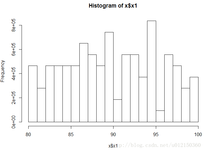
散点图绘制函数plot()
> plot(x1,x2)
> plot(x$x1,x$x2)

列联表分析——列联函数table(),柱状图绘制函数barplot()
> table(x$x1)

    80     81     82     83     84     85     86     87     88     89     90     91     92
 93001 372004 279003 465005 465005 465005 465005 651007 558006 465005 744008 186002 558006
    93     94     95     96     97     98     99    100
558006 372004 837009  93001 558006 465005 279003 372004
> barplot(table(x$x1)) 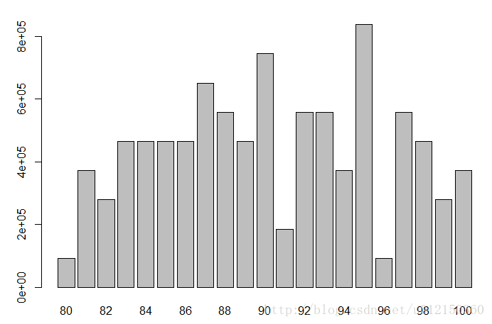
饼图——饼图绘制函数pie()
pie(table(x$x1))
箱尾图
- 箱子的上下横线为样本的25%和75%分位数
- 箱子中间横线为样本的中位数
- 上下延伸的直线称为尾线,尾线的尽头为最高值和最低值
- 异常值(超出一定阈值)——图中小圆点
> boxplot(x$x1,x$x2,x$x3)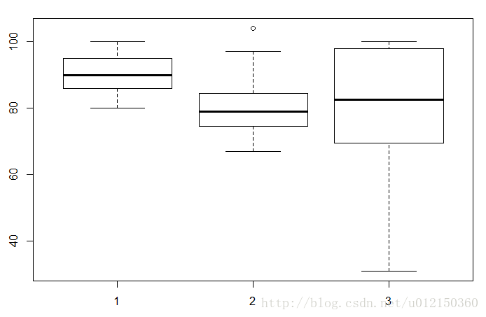
- 指定箱尾图的颜色和缺口
boxplot(x[1:100,2:4],col=c("red","green","blue"),notch = T) 
- 水平放置的箱尾图
boxplot(x$x1,x$x2,x$x3,horizontal = T)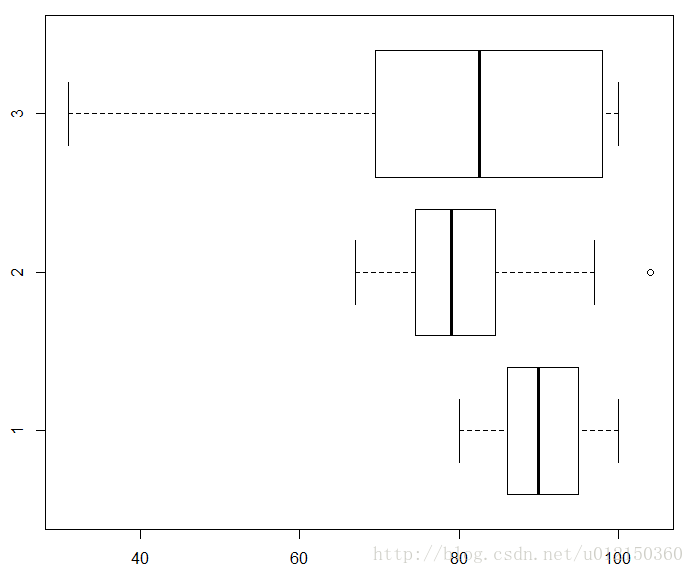
星相图
- 每个观测单位的数值表示为一个图形
- 每个图的每个角表示一个变量,字符串类型会标注在图的下方
- 角线的长度表达值得大小
> stars(x[c("x1","x2","x3")]) 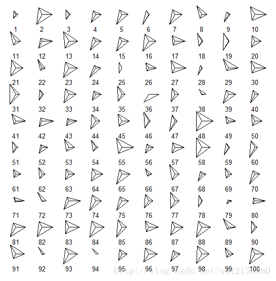
- 雷达图
用full=T/F 表示画整个圆还是半个圆,用draw.segment = T 表示画的是扇形
stars(x[c("x1","x2","x3")],full= T,draw.segment = T) 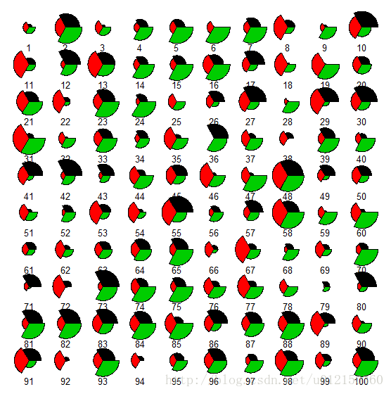
stars(x[c("x1","x2","x3")],full= F,draw.segment = T) 
脸谱图
安装aplpack包
> library("aplpack", lib.loc="D:/R_library")
> faces(x[c("x1","x2","x3")])
effect of variables:
 modified item       Var
 "height of face   " "x1"
 "width of face    " "x2"
 "structure of face" "x3"
 "height of mouth  " "x1"
 "width of mouth   " "x2"
 "smiling          " "x3"
 "height of eyes   " "x1"
 "width of eyes    " "x2"
 "height of hair   " "x3"
 "width of hair   "  "x1"
 "style of hair   "  "x2"
 "height of nose  "  "x3"
 "width of nose   "  "x1"
 "width of ear    "  "x2"
 "height of ear   "  "x3"
> - 用五官的宽带和高度来描述数值
- 人对脸谱高度敏感和强记忆
- 适合较少样本的情况
其他脸谱图
安装TeachingDemos包
> library(TeachingDemos)

Attaching package: ‘TeachingDemos’
The following objects are masked from ‘package:aplpack’:
    faces, slider

### 茎叶图
> stem(x$x2)
  The decimal point is 1 digit(s) to the right of the |
  6 | 14
  6 | 99
  7 | 000112222223444
  7 | 555666666777777788999
  8 | 0000111111122222222222333444
  8 | 55555567778999
  9 | 0000002223344
  9 | 55556
mistakes:
> stem(x$x1)

  The decimal point is at the |
   80 | 00000
   82 | 00000000
   84 | 0000000000
   86 | 000000000000
   88 | 00000000000
   90 | 0000000000
   92 | 000000000000
   94 | 0000000000000
   96 | 0000000
   98 | 00000000
  100 | 0000
改为:
> stem(x$x1,scale = 0.5)

  The decimal point is 1 digit(s) to the right of the |
   8 | 011112223333344444
   8 | 5555566666777777788888899999
   9 | 00000000112222223333334444
   9 | 555555555677777788888999
  10 | 0000
QQ图
- 可用于判断是否是正态分布
- 直线的斜率是标准差,截距是均值
- 点的散布越接近直线,则越接近正态分布
> qqnorm(x1)
> qqline(x1)
图中可看出x1不是正态分布
> qqnorm(x2)
> qqline(x2)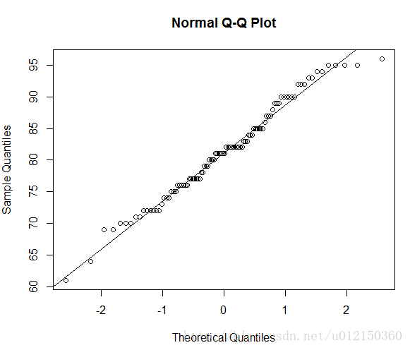
图中可看出x2很可能是正态分布
散点图
- 散点图的进一步设置
> plot(x$x1,x$x2,main="数学分析与线性代数成绩的关系",
+      xlab="数学分析",
+      ylab="线性代数",
+      xlim=c(0,100),
+      ylim=c(0,100),
+      xaxs="i",#Set x axis style as internal
+      yaxs="i", #Set x axis style as internal
+      col = "red", #Set the color of plotting symbol to red
+      pch=19 #Set the plotting symbol to filled dots
+ )

连线图
> a = c(2,3,4,5,6)
> b = c(4,7,8,9,12)
> plot(a,b,type = "l")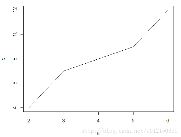
- 多条曲线的效果
> rain <- read.csv("D:/R_workspace/Dataguru/week2/rain.csv")
> rain
   Tokyo NewYork London Berlin
1     64     102     56     87
2     43      76     54     76
3     76      98     75     46
4     44      57     43     35
5     34      54     23     75
6     23      45     76     56
7     89      37     45     33
8     56      56     34     22
9    102      45     98      1
10   132      45    111     23
11    45      17    102    120
12    65      87     48     23
> plot(rain$Tokyo,type = "l",col = "red",ylim=c(0,300),main="Monthly Rainfall in major cities",xlab="Month of Year",ylab = "Rainfall(mm)",lwd=2)              # lwd 设置线宽
> lines(rain$NewYork,type = "l",col="blue",lwd=2)  #lines在原plot图的上面添加折线  lines称为低水平画图函数
> lines(rain$London,type = "l",col="green",lwd=2)
> lines(rain$Berlin,type = "l",col="orange",lwd=2)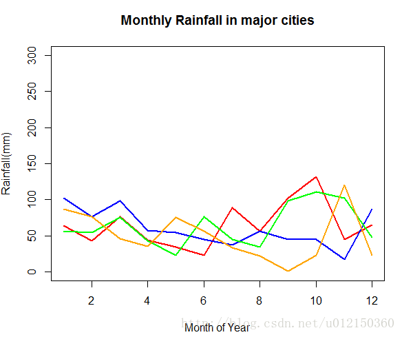
关于低水平作图和高水平作图 在薛毅书中P137-138
密度图
- 函数density()
> plot(density(rnorm(1000)))
R内置数据集
函数data()列出内置数据
data()例如
> mtcars
                     mpg cyl  disp  hp drat    wt  qsec vs am gear carb
Mazda RX4           21.0   6 160.0 110 3.90 2.620 16.46  0  1    4    4
Mazda RX4 Wag       21.0   6 160.0 110 3.90 2.875 17.02  0  1    4    4
Datsun 710          22.8   4 108.0  93 3.85 2.320 18.61  1  1    4    1
Hornet 4 Drive      21.4   6 258.0 110 3.08 3.215 19.44  1  0    3    1
Hornet Sportabout   18.7   8 360.0 175 3.15 3.440 17.02  0  0    3    2
Valiant             18.1   6 225.0 105 2.76 3.460 20.22  1  0    3    1
Duster 360          14.3   8 360.0 245 3.21 3.570 15.84  0  0    3    4
Merc 240D           24.4   4 146.7  62 3.69 3.190 20.00  1  0    4    2
Merc 230            22.8   4 140.8  95 3.92 3.150 22.90  1  0    4    2
Merc 280            19.2   6 167.6 123 3.92 3.440 18.30  1  0    4    4
Merc 280C           17.8   6 167.6 123 3.92 3.440 18.90  1  0    4    4
Merc 450SE          16.4   8 275.8 180 3.07 4.070 17.40  0  0    3    3
Merc 450SL          17.3   8 275.8 180 3.07 3.730 17.60  0  0    3    3
Merc 450SLC         15.2   8 275.8 180 3.07 3.780 18.00  0  0    3    3
Cadillac Fleetwood  10.4   8 472.0 205 2.93 5.250 17.98  0  0    3    4
Lincoln Continental 10.4   8 460.0 215 3.00 5.424 17.82  0  0    3    4
Chrysler Imperial   14.7   8 440.0 230 3.23 5.345 17.42  0  0    3    4
Fiat 128            32.4   4  78.7  66 4.08 2.200 19.47  1  1    4    1
Honda Civic         30.4   4  75.7  52 4.93 1.615 18.52  1  1    4    2
Toyota Corolla      33.9   4  71.1  65 4.22 1.835 19.90  1  1    4    1
Toyota Corona       21.5   4 120.1  97 3.70 2.465 20.01  1  0    3    1
Dodge Challenger    15.5   8 318.0 150 2.76 3.520 16.87  0  0    3    2
AMC Javelin         15.2   8 304.0 150 3.15 3.435 17.30  0  0    3    2
Camaro Z28          13.3   8 350.0 245 3.73 3.840 15.41  0  0    3    4
Pontiac Firebird    19.2   8 400.0 175 3.08 3.845 17.05  0  0    3    2
Fiat X1-9           27.3   4  79.0  66 4.08 1.935 18.90  1  1    4    1
Porsche 914-2       26.0   4 120.3  91 4.43 2.140 16.70  0  1    5    2
Lotus Europa        30.4   4  95.1 113 3.77 1.513 16.90  1  1    5    2
Ford Pantera L      15.8   8 351.0 264 4.22 3.170 14.50  0  1    5    4
Ferrari Dino        19.7   6 145.0 175 3.62 2.770 15.50  0  1    5    6
Maserati Bora       15.0   8 301.0 335 3.54 3.570 14.60  0  1    5    8
Volvo 142E          21.4   4 121.0 109 4.11 2.780 18.60  1  1    4    2
热力图
- 利用内置的mtcars数据集绘制
> heatmap(as.matrix(mtcars),Rowv = NA,Colv = NA,col = heat.colors(256),scale = "column",margins = c(2,8),main = "Car characteristics by Model") #要先把数据框转化成矩阵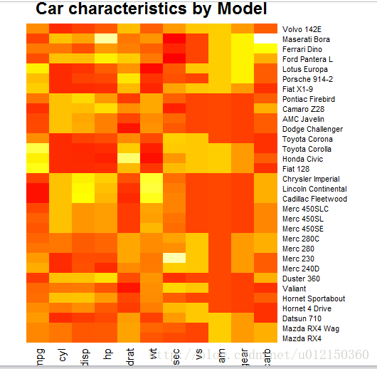
Iris(鸢尾花)数据集
- Sepal 花萼
- Petal 花瓣
- Species 种属
> iris
    Sepal.Length Sepal.Width Petal.Length Petal.Width    Species
1            5.1         3.5          1.4         0.2     setosa
2            4.9         3.0          1.4         0.2     setosa
3            4.7         3.2          1.3         0.2     setosa
4            4.6         3.1          1.5         0.2     setosa
5            5.0         3.6          1.4         0.2     setosa
6            5.4         3.9          1.7         0.4     setosa
 ………………
147          6.3         2.5          5.0         1.9  virginica
148          6.5         3.0          5.2         2.0  virginica
149          6.2         3.4          5.4         2.3  virginica
150          5.9         3.0          5.1         1.8  virginica
向日葵散点图
- 用来克服散点图中数据点重叠问题
- 在有重叠的地方用一朵“向日葵”的花瓣数目来表示重叠数据的个数
> sunflowerplot(iris[,3:4],col = "gold",seg.col = "gold") #col指定点的颜色 seg.col指定放射线的颜色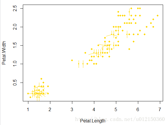
散点图集
- 遍历样本中全部的变量配对画出二元图
- 直观地了解所有变量之间的关系
> pairs(iris[,1:4])
用plot也可以实现同样的效果
> plot(iris[,1:4],main="Relationships between characteristics of iris flowers",pch=19,col="blue",cex=0.9)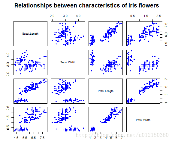
- 利用par()在同一个device()中输出多个散点图
- Par命令博大精深,用于设置绘图参数,help(par)
> par(mfrow=c(3,1))
> plot(x1,x2);plot(x2,x3);plot(x3,x1) 
关于绘图参数
- help(par)
- 有哪些颜色?colors()
> colors()- 绘图设备
dev.new()        #新建图形窗
dev.cur()        #显示目前的窗口编号
dev.list()       #窗口的列表
dev.next(which = dev.cur())
dev.prev(which = dev.cur())
dev.off(which = dev.cur())
dev.set(which = dev.next())
graphics.off()
关于绘图参数
三维散点图
- 安装scatterplot3d包
> library(scatterplot3d)
> scatterplot3d(x[2:4])
- 三维作图
> x<-y<-seq(-2*pi,2*pi,pi/15)
> f<-function(x,y) sin(x)*sin(y)
> z<-outer(x,y,f)
> contour(x,y,z,col = "blue")
> persp(x,y,z,theta = 30,phi = 30,expand = 0.7,col = "lightblue")
调和曲线图
- unison.r的代码
- 自定义函数
- 条和曲线用于聚类半段非常方便
> source("D:/R_workspace/Dataguru/week2/unison.R")
> unison(x[2:4])
地图
- 安装maps包
> library(maps)
> map("state",interior = FALSE)
> map("state",boundary = FALSE,col = "red",add = TRUE)
> map("world",fill = TRUE,col=heat.colors(10))
R实验:社交数据可视化
- 先下载安装maps包和geosphere包并加载
library(maps)
library(geosphere)- 画出美国地图
map("state")
- 画出世界地图
> map("world")
- 通过设置坐标范围使焦点集中在美国周边,并期望设置一些有关颜色
> xlim <- c(-171.738281,-56.601563)
> ylim <- c(12.039321,71.856229)
> map("world",col = "#f2f2f2",fill = TRUE,bg="white",lwd=0.05,xlim = xlim,ylim = ylim)
> 
- 画一条弧线连线,表示社交关系
> library("geosphere", lib.loc="D:/R_library")
> lat_me <- 45.21300
> lon_me <- -68.906250
> inter <- gcIntermediate(c(lon_ca,lat_ca),c(lon_me,lat_me),n=50,addStartEnd=TRUE)
> lines(inter)
- 继续画弧线
> lat_tx <- 29.954935
> lon_tx <- -98.701172
> inter2 <- gcIntermediate(c(lon_ca,lat_ca),c(lon_tx,lat_tx),n=50,addStartEnd=TRUE)
> lines(inter2,col="red")
- 装载数据
> airports <- read.csv("http://datasets.flowingdata.com/tuts/maparcs/airports.csv",header = TRUE)
> flights <- read.csv("http://datasets.flowingdata.com/tuts/maparcs/flights.csv",header = TRUE,as.is = TRUE)- 画出多重联系
> map("world",col = "#f2f2f2",fill=TRUE,bg="white",lwd=0.05,xlim=xlim,ylim=ylim)
> fsub <- flights[flights$airline == "AA",]
> for(j in 1:length(fsub$airline)){
+ air1 <- airports[airports$iata == fsub[j,]$airport1,]
+ air2 <- airports[airports$iata == fsub[j,]$airport2,]
+ inter <- gcIntermediate(c(air1[1,]$long,air1[1,]$lat),c(air2[1,]$long,air2[1,]$lat),n=100,addStartEnd=TRUE)
+ lines(inter,col = "black",lwd=0.8)
+ } 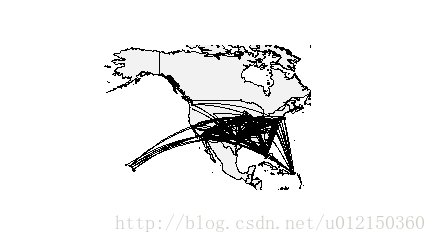
画map链接:http://flowingdata.com/2011/05/11/how-to-map-connections-with-great-circles/