Feb20-paper reading-Convolutional Recurrent Neural Networks for Dynamic MR Image Reconstruction

1. Convolutional Recurrent Neural Networks for Dynamic MR Image Reconstruction

MY NOTES:
结合之前读过类似的image denoising 或者图像重建的文章，最后都是转化成一个优化问题，在上次讲过的论文中，作者使用稀疏矩阵的方法来解决优化问题，最后的优化问题还是转化成一个迭代问题求解。

在本文中，同样优化问题改编为两部迭代求解最优化的问题，但是在迭代中，迭代的每一步，作者引入CRNN的框架，不再需要提前确定一些超参数来求解，完全依靠模型自己去训练和学习。
其中的CRNN block 可以作为梯度下降求解最优化问题的梯度下降迭代项。

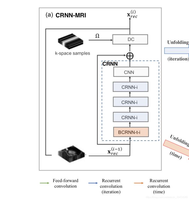
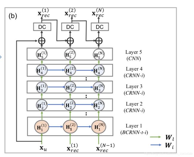
本文最主要的就是图片中的那个结构。

Object：Accelerate the data acquisition of dynamic MRI.
The key issue of the problem is how to exploit the temporal correlations of the MR sequences to resolve aliasing artefacts.

The image can be reconstructed by solving an optimisation problem.

However, the challenges of these optimisation based approaches are the following:

• firstly, the regularisation functions and their hyper-parameters must be carefully selected, which are problem-specific and non-trivial.For example, over-imposing sparsity or L1 penalties can lead to cartoon-like/staircase artefacts.
• Secondly, the reconstruction speeds of these methods are often slow due to requirement to solve iterative algorithms. Proposing a robust iterative algorithm is still an active area of research.

Deep learning based methods are gaining popularity for their accuracy and efficiency.

Unlike traditional approaches, the prior information and regularisation are learnt implicitly from data, without having to specify them in the training objective.

In this work, our contribution:

we propose a novel convolutional recurrent neural network (CRNN) method to reconstruct high quality dynamic MR image sequences from under-sampled data, termed CRNN-MRI.

1. Firstly, we formulate a general optimisation problem for solving accelerated dynamic MRI based on variable splitting and alternate minimisation.

We then show how this algorithm can be seen as a network architecture.
In particular, the proposed method consists of a CRNN block which acts as the proximal operator and a data consistency layer corresponding to the classical data fidelity term.
In addition, the CRNN block employs recurrent connections across each iteration step, allowing reconstruction information to be shared across the multiple iterations of the process.

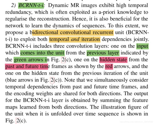
2. Secondly, we incorporate bidirectional convolutional recurrent units evolving over time to exploit the temporal dependency of the dynamic sequences and effectively propagate the contextual information across time frames of the input.

As a consequence, the unique CRNN architecture jointly learns representations in a recurrent fashion evolving over both time sequences as well as iterations of the reconstruction process, effectively combining the benefits of traditional iterative methods and deep learning.

Model: CRNN-MRI

A: Problem Formulation

x $\in$ $C^D$(complexed-valued MR images to be reconstructed)
D = $D_x{D}_{y}T$
y $\in C^M$ (M << D)
y is the under-sampled k-space measurements

$D_x{D}_y$ is the width and height of frame;
T is the number of frames.
our problem: is to reconstruct x from y

Model:

argmin${}_x$ $R(x)+\lambda ||y-F_{u}x|{|}_2^2$ (1)
$F_u$: an undersampling Fourier encoding matrix
R: regularisation terms on x
$\lambda$: adjustment of data fidelity.

Always we can use variable splitting technique to handle the model above.

We introduce another variable z, and (1) can be transformed to (2)

argmin${}_{x,z}$ $R(z)+\lambda ||y-F_{u}x|{|}_2^2$ + $\mu ||x-z|{|}_2^2$                      ~~~~~~~~~~~~~~~~~~~~                     (2)
$\mu$: penalty parameter

Then we apply alternate minimisation over x and z, and then we get:
$z^{(i+1)}$= argmin${}_z$ R(z) + $\mu ||x-z|{|}_2^2$                                           ~~~~~~~~~~~~~~~~~~~~~~~~~~~~~~~~~~~~~~~~~                                          (3a)
$x^{(i+1)}=argmi{n}_x\lambda ||y-F_{u}x|{|}_2^2+\mu ||x-z^{(i+1)}|{|}_2^2$               ~~~~~~~~~~~~~              (3b)

Then during our iteration, $x^{(0)}=x_{\mu }=F_u^{H}y$, which is a zero-filled reconstruction taken as an initialisation.
z can be seen as an intermediate state of optimisation process.

For MRI reconstruction, 3b is often regarded as a data consistency(DC) steps.

In this formula, F is full Fourier encoding matrix.
${\lambda }_0=\frac{\lambda }{\mu }$ is ratio of regularisation parameters.
$\Lambda$ is diagonal matrix.

But in Deep-ADMM method , they unroll the traditional optimisation algorithm to.
$x^{(0)}\to z^{(1)}\to x^{(1)}\to z^{(2)}\to x^{(2)}\to ........\to z^{(N)}\to x^{(N)}$
during this iteration, each state transition at stage(i) is an operation such as convolutions independently parametered by $\theta$.

But our model use CRNN, in which, each stage(i), as a learnt, recurrent, forward encoding step.
$f_i$ $(x^{(i-1)},z^{(i-1)};\theta ,y,\lambda ,\Omega )$

B: CNN for MRI reconstruction

$x_{rec}=f_N(f_{(N-1)}(.....f_1(x_{\mu })))$
$x_{rec}$: prediction of the network
$x_{\mu }$: sequence of under-sampled image with length T and also is the input of the network
$f_i(x_{\mu };\theta ,\lambda ,\Omega )$ is the network function for each iteration of optimization step.
N is the number of iterations.

The model can be written as:
$x_{rnn}^{(i)}=x_{rec}^{(i-1)}+CRNN(x_{rec}^{(i-1)})$
$x_{rec}^{(i)}$ = DC($x_{rnn}^{(i)};y,{\lambda }_0,\Omega$)

DC can be treated as a network layer.

CRNN block is to encode the update steps, and can be seen as one step of gradient descent in object minimisation.
this block can be seen as the distance required to move to the next state in the network.

CRNN: is the learnable block,
$x_{rec}^{(i)}$ is progressive reconstruction of the under-sampled image $x_{\mu }$ at iteration i with $x_{rec}^{(0)}=x_{\mu }$.
$x_{rnn}^{(i)}$ is the intermediate reconstruction image before the DC layer.
$x_{rec}\approx x$
$x_{rnn}\approx z$ in equation 3
y is the acquired k-space sample.
we want to reconstruct x from y.
each state: CRNN update its internal state H given an input.
Furthermore, CRNN block comprised of 5 components:

1. bidirectional convolutional recurrent units evolving over time and iterations (BCRNN-t-i)

2. convolutional recurrent units evolving over iterations only (CRNN-i)

3. 2D convolutional neural network (CNN)
4. residual connection
5. DC layers.

That is the end of the model.

Appendix:
The example about bidirectional RNN