【图像去噪】小波变换+Contourlet变换+PCA图像去噪【含Matlab源码 610期】
⛄一、图像去噪及滤波简介
1 图像去噪
1.1 图像噪声定义
噪声是干扰图像视觉效果的重要因素,图像去噪是指减少图像中噪声的过程。噪声分类有三种:加性噪声,乘性噪声和量化噪声。我们用f(x,y)表示图像,g(x,y)表示图像信号,n(x,y)表示噪声。
图像去噪是指减少数字图像中噪声的过程。现实中的数字图像在数字化和传输过程中常受到成像设备与外部环境噪声干扰等影响,称为含噪图像或噪声图像。去噪是图像处理研究中的一个重点内容。在图像的获取、传输、发送、接收、复制、输出等过程中,往往都会产生噪声,其中的椒盐噪声是比较常见的一种噪声,它属于加性噪声。
1.2 图像噪声来源
(1)图像获取过程中
图像传感器CCD和CMOS采集图像过程中受传感器材料属性、工作环境、电子元器件和电路结构等影响,会引入各种噪声。
(2)图像信号传输过程中
传输介质和记录设备等的不完善,数字图像在其传输记录过程中往往会受到多种噪声的污染。
1.3 噪声分类
噪声按照不同的分类标准可以有不同的分类形式:
基于产生原因:内部噪声,外部噪声。
基于噪声与信号的关系:
加性噪声:加性噪声和图像信号强度是不相关的,这类带有噪声的图像g可看成为理想无噪声图像f与噪声n之和:
g = f + n;
乘性嗓声:乘性噪声和图像信号是相关的,往往随图像信号的变化而变化,载送每一个象素信息的载体的变化而产生的噪声受信息本身调制。在某些情况下,如信号变化很小,噪声也不大。为了分析处理方便,常常将乘性噪声近似认为是加性噪声,而且总是假定信号和噪声是互相统计独立。
g = f + f*n
按照基于统计后的概率密度函数:
是比较重要的,主要因为引入数学模型这就有助于运用数学手段去除噪声。在不同场景下噪声的施加方式都不同,由于在外界的某种条件下,噪声下图像-原图像(没有噪声时)的概率密度函数(统计结果)服从某种分布函数,那么就把它归类为相应的噪声。下面将具体说明基于统计后的概率密度函数的噪声分类及其消除方式。
1.4 图像去噪算法的分类
(1)空间域滤波
空域滤波是在原图像上直接进行数据运算,对像素的灰度值进行处理。常见的空间域图像去噪算法有邻域平均法、中值滤波、低通滤波等。
(2)变换域滤波
图像变换域去噪方法是对图像进行某种变换,将图像从空间域转换到变换域,再对变换域中的变换系数进行处理,再进行反变换将图像从变换域转换到空间域来达到去除图像嗓声的目的。将图像从空间域转换到变换域的变换方法很多,如傅立叶变换、沃尔什-哈达玛变换、余弦变换、K-L变换以及小波变换等。而傅立叶变换和小波变换则是常见的用于图像去噪的变换方法。
(3)偏微分方程
偏微分方程是近年来兴起的一种图像处理方法,主要针对低层图像处理并取得了很好的效果。偏微分方程具有各向异性的特点,应用在图像去噪中,可以在去除噪声的同时,很好的保持边缘。偏微分方程的应用主要可以分为两类:一种是基本的迭代格式,通过随时间变化的更新,使得图像向所要得到的效果逐渐逼近,这种算法的代表为Perona和Malik的方程,以及对其改进后的后续工作。该方法在确定扩散系数时有很大的选择空间,在前向扩散的同时具有后向扩散的功能,所以,具有平滑图像和将边缘尖锐化的能力。偏微分方程在低噪声密度的图像处理中取得了较好的效果,但是在处理高噪声密度图像时去噪效果不好,而且处理时间明显高出许多。
(4)变分法
另一种利用数学进行图像去噪方法是基于变分法的思想,确定图像的能量函数,通过对能量函数的最小化工作,使得图像达到平滑状态,现在得到广泛应用的全变分TV模型就是这一类。这类方法的关键是找到合适的能量方程,保证演化的稳定性,获得理想的结果。
形态学噪声滤除器将开与闭结合可用来滤除噪声,首先对有噪声图像进行开运算,可选择结构要素矩阵比噪声尺寸大,因而开运算的结果是将背景噪声去除;再对前一步得到的图像进行闭运算,将图像上的噪声去掉。据此可知,此方法适用的图像类型是图像中的对象尺寸都比较大,且没有微小细节,对这类图像除噪效果会较好。
⛄二、部分源代码
function y = sefilter2(x, f1, f2, extmod, shift)
% SEFILTER2 2D seperable filtering with extension handling
%
% y = sefilter2(x, f1, f2, [extmod], [shift])
%
% Input:
% x: input image
% f1, f2: 1-D filters in each dimension that make up a 2D seperable filter
% extmod: [optional] extension mode (default is ‘per’)
% shift: [optional] specify the window over which the
% convolution occurs. By default shift = [0; 0].
%
% Output:
% y: filtered image of the same size as the input image:
% Y(z1,z2) = X(z1,z2)*F1(z1)*F2(z2)*z1shift(1)*z2shift(2)
%
% Note:
% The origin of the filter f is assumed to be floor(size(f)/2) + 1.
% Amount of shift should be no more than floor((size(f)-1)/2).
% The output image has the same size with the input image.
%
% See also: EXTEND2, EFILTER2
if ~exist(‘extmod’, ‘var’)
extmod = ‘per’;
end
if ~exist(‘shift’, ‘var’)
shift = [0; 0];
end
% Make sure filter in a row vector
f1 = f1(‘;
f2 = f2(’;
% Periodized extension
lf1 = (length(f1) - 1) / 2;
lf2 = (length(f2) - 1) / 2;
y = extend2(x, floor(lf1) + shift(1), ceil(lf1) - shift(1), …
floor(lf2) + shift(2), ceil(lf2) - shift(2), extmod);
% Seperable filter
y = conv2(f1, f2, y, ‘valid’);
function x = pprec(p0, p1, type)
% PPREC Parallelogram Polyphase Reconstruction
%
% x = pprec(p0, p1, type)
%
% Input:
% p0, p1: two parallelogram polyphase components of the image
% type: one of {1, 2, 3, 4} for selecting sampling matrices:
% P1 = [2, 0; 1, 1]
% P2 = [2, 0; -1, 1]
% P3 = [1, 1; 0, 2]
% P4 = [1, -1; 0, 2]
%
% Output:
% x: reconstructed image
%
% Note:
% These sampling matrices appear in the directional filterbank:
% P1 = R1 * Q1
% P2 = R2 * Q2
% P3 = R3 * Q2
% P4 = R4 * Q1
% where R’s are resampling matrices and Q’s are quincunx matrices
%
% Also note that R1 * R2 = R3 * R4 = I so for example,
% upsample by R1 is the same with down sample by R2
%
% See also: PPDEC
% Parallelogram polyphase decomposition by simplifying sampling matrices
% using the Smith decomposition of the quincunx matrices
[m, n] = size(p0);
switch type
case 1 % P1 = R1 * Q1 = D1 * R3
x = zeros(2*m, n);
x(1:2:end, :) = resamp(p0, 4);
x(2:2:end, [2:end, 1]) = resamp(p1, 4);

case 2	% P2 = R2 * Q2 = D1 * R4
x = zeros(2*m, n);

x(1:2:end, :) = resamp(p0, 3);
x(2:2:end, :) = resamp(p1, 3);

case 3	% P3 = R3 * Q2 = D2 * R1
x = zeros(m, 2*n);

x(:, 1:2:end) = resamp(p0, 2);
x([2:end, 1], 2:2:end) = resamp(p1, 2);

case 4	% P4 = R4 * Q1 = D2 * R2
x = zeros(m, 2*n);

x(:, 1:2:end) = resamp(p0, 1);
x(:, 2:2:end) = resamp(p1, 1);

otherwise
error('Invalid argument type');
end
function x = pdfbrec(y, pfilt, dfilt)
% PDFBREC Pyramid Directional Filterbank Reconstruction
%
% x = pdfbrec(y, pfilt, dfilt)
%
% Input:
% y: a cell vector of length n+1, one for each layer of
% subband images from DFB, y{1} is the low band image
% pfilt: filter name for the pyramid
% dfilt: filter name for the directional filter bank
%
% Output:
% x: reconstructed image
%
% See also: PFILTERS, DFILTERS, PDFBDEC
n = length(y) - 1;
if n <= 0
x = y{1};
else
% Recursive call to reconstruct the low band
xlo = pdfbrec(y(1:end-1), pfilt, dfilt);
% Get the pyramidal filters from the filter name
[h, g] = pfilters(pfilt);

% Process the detail subbands
if length(y{end}) ~= 3
    % Reconstruct the bandpass image from DFB

    % Decide the method based on the filter name
    switch dfilt
        case {'pkva6', 'pkva8', 'pkva12', 'pkva'}
            % Use the ladder structure (much more efficient)
            xhi = dfbrec_l(y{end}, dfilt);

        otherwise
            % General case
            xhi = dfbrec(y{end}, dfilt);
    end

    x = lprec(xlo, xhi, h, g);

else
    % Special case: length(y{end}) == 3
    % Perform one-level 2-D critically sampled wavelet filter bank
    x = wfb2rec(xlo, y{end}{1}, y{end}{2}, y{end}{3}, h, g);
end
end
function x = pprec(p0, p1, type)
% PPREC Parallelogram Polyphase Reconstruction
%
% x = pprec(p0, p1, type)
%
% Input:
% p0, p1: two parallelogram polyphase components of the image
% type: one of {1, 2, 3, 4} for selecting sampling matrices:
% P1 = [2, 0; 1, 1]
% P2 = [2, 0; -1, 1]
% P3 = [1, 1; 0, 2]
% P4 = [1, -1; 0, 2]
%
% Output:
% x: reconstructed image
%
% Note:
% These sampling matrices appear in the directional filterbank:
% P1 = R1 * Q1
% P2 = R2 * Q2
% P3 = R3 * Q2
% P4 = R4 * Q1
% where R’s are resampling matrices and Q’s are quincunx matrices
%
% Also note that R1 * R2 = R3 * R4 = I so for example,
% upsample by R1 is the same with down sample by R2
%
% See also: PPDEC
% Parallelogram polyphase decomposition by simplifying sampling matrices
% using the Smith decomposition of the quincunx matrices
[m, n] = size(p0);
switch type
case 1 % P1 = R1 * Q1 = D1 * R3
x = zeros(2*m, n);
x(1:2:end, :) = resamp(p0, 4);
x(2:2:end, [2:end, 1]) = resamp(p1, 4);

case 2	% P2 = R2 * Q2 = D1 * R4
x = zeros(2*m, n);

x(1:2:end, :) = resamp(p0, 3);
x(2:2:end, :) = resamp(p1, 3);

case 3	% P3 = R3 * Q2 = D2 * R1
x = zeros(m, 2*n);

x(:, 1:2:end) = resamp(p0, 2);
x([2:end, 1], 2:2:end) = resamp(p1, 2);

case 4	% P4 = R4 * Q1 = D2 * R2
x = zeros(m, 2*n);

x(:, 1:2:end) = resamp(p0, 1);
x(:, 2:2:end) = resamp(p1, 1);

otherwise
error('Invalid argument type');
end
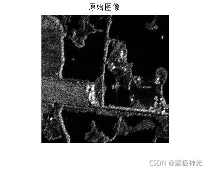
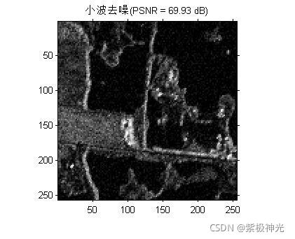
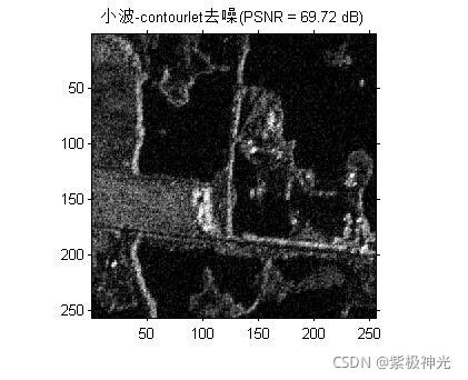
⛄三、运行结果


⛄四、matlab版本及参考文献
1 matlab版本
2014a
2 参考文献
[1] 蔡利梅.MATLAB图像处理——理论、算法与实例分析[M].清华大学出版社,2020.
[2]杨丹,赵海滨,龙哲.MATLAB图像处理实例详解[M].清华大学出版社,2013.
[3]周品.MATLAB图像处理与图形用户界面设计[M].清华大学出版社,2013.
[4]刘成龙.精通MATLAB图像处理[M].清华大学出版社,2015.
[5]基于matlab的传统算法图像去噪的实现原理
3 备注
简介此部分摘自互联网,仅供参考,若侵权,联系删除