Batch Normalization和Dropout

目录

导包和处理数据

BatchNorm

forward

backward

训练BatchNorm并显示结果

 Batch Normalization 和初始化

 Batch Normalization 和 Batch Size

 Layer Normalization

Layer Normalization 和 Batch Size

卷积层的batch norm--spatial batchnorm

Spatial Group Normalization

dropout

Regularization Experiment

 Solver和网络

solver

 网络

网络用到的辅助函数（各层）

损失函数

---

The authors of [1] hypothesize that the shifting distribution of features inside deep neural networks may make training deep networks more difficult. To overcome this problem, they propose to insert into the network layers that normalize batches. At training time, such a layer uses a minibatch of data to estimate the mean and standard deviation of each feature. These estimated means and standard deviations are then used to center and normalize the features of the minibatch. A running average of these means and standard deviations is kept during training, and at test time these running averages are used to center and normalize features.

It is possible that this normalization strategy could reduce the representational power of the network, since it may sometimes be optimal for certain layers to have features that are not zero-mean or unit variance. To this end, the batch normalization layer includes learnable shift and scale parameters for each feature dimension.

Sergey Ioffe and Christian Szegedy, "Batch Normalization: Accelerating Deep Network Training by Reducing Internal Covariate Shift", ICML 2015.

导包和处理数据

# Setup cell.
import time
import numpy as np
import matplotlib.pyplot as plt
from cs231n.data_utils import get_CIFAR10_data
from cs231n.gradient_check import eval_numerical_gradient, eval_numerical_gradient_array

%matplotlib inline
plt.rcParams["figure.figsize"] = (10.0, 8.0)  # Set default size of plots.
plt.rcParams["image.interpolation"] = "nearest"
plt.rcParams["image.cmap"] = "gray"

%load_ext autoreload
%autoreload 2

def rel_error(x, y):
    """Returns relative error."""
    return np.max(np.abs(x - y) / (np.maximum(1e-8, np.abs(x) + np.abs(y))))

def print_mean_std(x,axis=0):
    print(f"  means: {x.mean(axis=axis)}")
    print(f"  stds:  {x.std(axis=axis)}\n")
    
# Load the (preprocessed) CIFAR-10 data.
data = get_CIFAR10_data()
for k, v in list(data.items()):
    print(f"{k}: {v.shape}")

BatchNorm

forward

The outputs from the last layer of the network should not be normalized. 

def batchnorm_forward(x, gamma, beta, bn_param):
    """
    During training the sample mean and (uncorrected) sample variance are
    computed from minibatch statistics and used to normalize the incoming data.
    During training we also keep an exponentially decaying running mean of the
    mean and variance of each feature, and these averages are used to normalize
    data at test-time.

    At each timestep we update the running averages for mean and variance using
    an exponential decay based on the momentum parameter:

    running_mean = momentum * running_mean + (1 - momentum) * sample_mean
    running_var = momentum * running_var + (1 - momentum) * sample_var

    Note that the batch normalization paper suggests a different test-time
    behavior: they compute sample mean and variance for each feature using a
    large number of training images rather than using a running average. For
    this implementation we have chosen to use running averages instead since
    they do not require an additional estimation step; the torch7
    implementation of batch normalization also uses running averages.

    Input:
    - x: Data of shape (N, D)
    - gamma: Scale parameter of shape (D,)
    - beta: Shift paremeter of shape (D,)
    - bn_param: Dictionary with the following keys:
      - mode: 'train' or 'test'; required
      - eps: Constant for numeric stability
      - momentum: Constant for running mean / variance.
      - running_mean: Array of shape (D,) giving running mean of features
      - running_var Array of shape (D,) giving running variance of features

    Returns a tuple of:
    - out: of shape (N, D)
    - cache: A tuple of values needed in the backward pass
    """
    mode = bn_param["mode"]
    eps = bn_param.get("eps", 1e-5)
    momentum = bn_param.get("momentum", 0.9)

    N, D = x.shape
    running_mean = bn_param.get("running_mean", np.zeros(D, dtype=x.dtype))
    running_var = bn_param.get("running_var", np.zeros(D, dtype=x.dtype))

    out, cache = None, None
    if mode == "train":
        x_mean = np.mean(x, axis = 0)
        x_var = np.var(x, axis = 0) + eps
        x_norm = (x - x_mean) / np.sqrt(x_var)
        out = x_norm * gamma  + beta  #  (N, D)
        cache = (x, x_norm, gamma, x_mean, x_var)
        
        # Store the updated running means back into bn_param
        bn_param["running_mean"] = momentum * running_mean + (1 - momentum) * x_mean
        bn_param["running_var"] = momentum * running_var + (1 - momentum) * x_var        

    elif mode == "test":
        x_norm = (x - running_mean) / np.sqrt(running_var + eps) 
        out = gamma * x_norm + beta
    else:
        raise ValueError('Invalid forward batchnorm mode "%s"' % mode)

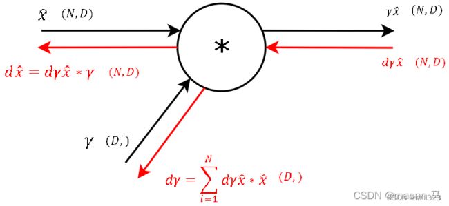
    return out, cache

backward

可以参考：

【cs231n】Batchnorm及其反向传播_JoeYF_的博客-CSDN博客_batchnorm反向传播

Batch Normalization的反向传播解说_macan_dct的博客-CSDN博客_batchnorm反向传播

Understanding the backward pass through Batch Normalization Layer

理解Batch Normalization（批量归一化）_坚硬果壳_的博客-CSDN博客

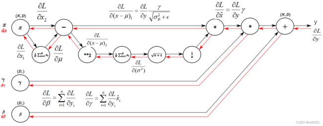
步骤9：

步骤8：

步骤7：

步骤6：

步骤5：

步骤4：

步骤3：

步骤2：

步骤1：

步骤0：

复杂版

def batchnorm_backward(dout, cache):
    """  
    Inputs:
    - dout: Upstream derivatives, of shape (N, D)
    - cache: Variable of intermediates from batchnorm_forward.

    Returns a tuple of:
    - dx: Gradient with respect to inputs x, of shape (N, D)
    - dgamma: Gradient with respect to scale parameter gamma, of shape (D,)
    - dbeta: Gradient with respect to shift parameter beta, of shape (D,)
    """
    dx, dgamma, dbeta = None, None, None

    x, x_norm, gamma, mean, var = cache
    N, D = dout.shape
    
    dbeta = np.sum(dout, axis = 0)
    dgamma = np.sum(dout * x_norm, axis = 0)  #  (N, D) * (N, D)
    # 注意求dgamma的时候没有使用矩阵乘法。在FC层的反向传播需要中矩阵乘法
    #可能因为正向传播的时候就没有使用真正的矩阵乘法，用的是(N, D) * (D,)
         
    dx_norm = dout * gamma  # (N, D) * (D,) x_norm是归一处理后的x      
    x_mu = x - mean
    std = np.sqrt(var)  # var已经包含了eps
    ivar = 1 / std # (D,)   
    # 求x_norm的式子中，分子分母中都含有x_mu，先求对这个x_mu的导数
    # 将std的倒数视作一个乘数
    dxmu1 = dx_norm * ivar  # (N, D) * (D,) 
    divar = np.sum(dx_norm * x_mu, axis = 0)  # 
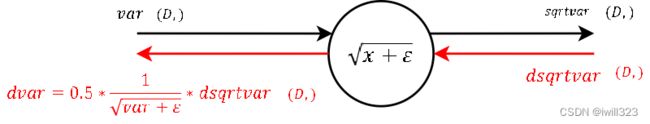
    dsqrtvar = - 1/ (std ** 2) * divar  # 倒数对根号项的导数 根号项正是std
    dvar = 0.5 / std * dsqrtvar  # 根号项对var(根号项中非eps项)的导数
    dsquare = 1/N * np.ones((N, D)) * dvar  #求var时对（N,D）矩阵进行了求列平均操作
    dxmu2 = 2 * x_mu * dsquare # 平方项对x_mu求导
    dx1 = dxmu1 + dxmu2
    
    #下面求x_mu对x的导数，注意平均值mu也是x的函数，所以导数是一个和
    # 先对mu求导，然后mu对x求导    
    dmu = -1 * np.sum(dx1, axis = 0)  # (D,)  广播的反向传播
    dx2 = 1/N * np.ones((N, D)) * dmu  # 求mu时采用了求平均的操作
    dx = dx1 + dx2
    return dx, dgamma, dbeta

 快速版

def batchnorm_backward_alt(dout, cache):
    """
    derive a simple expression for the backward pass.   

    """
    dx, dgamma, dbeta = None, None, None
    x, x_norm, gamma, mean, var = cache
    std = np.sqrt(var)
    
    dgamma = np.sum(dout * x_norm, axis = 0)  #  (N, D) * (N, D)
    dbeta = np.sum(dout, axis = 0)
    
    N = 1.0 * x.shape[0]
    dfdu = dout * gamma
    # 将x_norm拆成x，mu，var三项，分别对x求导，然后加起来
    dfdv = np.sum(dfdu * (x - mean) * -0.5 * var ** -1.5, axis = 0) # f对var求导   
    dfdw = np.sum(dfdu * -1 / std, axis = 0) + \
        dfdv * np.sum(-2/N * (x - mean), axis = 0)  # f对mu求导，包括var项对mu求导
    dx = dfdu / std + dfdv * 2/N * (x - mean) + dfdw / N  # 三项分别对x求导并求和

    '''
    # 也可以用下面方式算，看不懂
    N = dout.shape[0]         
    dfdz = dout * gamma                          # 下面用 z 指代 x_norm  [NxD]
    dfdz_sum = np.sum(dfdz,axis=0)                                      #[1xD]
    dx = dfdz - dfdz_sum/N - np.sum(dfdz * x_norm,axis=0) * x_norm/N    #[NxD]
    dx /= std
    '''
    return dx, dgamma, dbeta

训练BatchNorm并显示结果

训练

np.random.seed(231)

# Try training a very deep net with batchnorm.
hidden_dims = [100, 100, 100, 100, 100]

num_train = 1000
small_data = {
  'X_train': data['X_train'][:num_train],
  'y_train': data['y_train'][:num_train],
  'X_val': data['X_val'],
  'y_val': data['y_val'],
}

weight_scale = 2e-2
bn_model = FullyConnectedNet(hidden_dims, weight_scale=weight_scale, normalization='batchnorm')
model = FullyConnectedNet(hidden_dims, weight_scale=weight_scale, normalization=None)

print('Solver with batch norm:')
bn_solver = Solver(bn_model, small_data,
                num_epochs=10, batch_size=50,
                update_rule='adam',
                optim_config={
                  'learning_rate': 1e-3,
                },
                verbose=True,print_every=20)
bn_solver.train()

print('\nSolver without batch norm:')
solver = Solver(model, small_data,
                num_epochs=10, batch_size=50,
                update_rule='adam',
                optim_config={
                  'learning_rate': 1e-3,
                },
                verbose=True, print_every=20)
solver.train()

Solver with batch norm:
(Iteration 1 / 200) loss: 2.340975
(Epoch 0 / 10) train acc: 0.107000; val_acc: 0.115000
(Epoch 1 / 10) train acc: 0.314000; val_acc: 0.266000
……
(Epoch 9 / 10) train acc: 0.767000; val_acc: 0.318000
(Iteration 181 / 200) loss: 0.888016
(Epoch 10 / 10) train acc: 0.808000; val_acc: 0.333000

Solver without batch norm:
(Iteration 1 / 200) loss: 2.302332
(Epoch 0 / 10) train acc: 0.129000; val_acc: 0.131000
……
(Iteration 161 / 200) loss: 1.034116
(Epoch 9 / 10) train acc: 0.654000; val_acc: 0.342000
(Iteration 181 / 200) loss: 0.905795
(Epoch 10 / 10) train acc: 0.714000; val_acc: 0.331000

显示结果

def plot_training_history(title, label, baseline, bn_solvers, plot_fn, bl_marker='.', 
                          bn_marker='.', labels=None):
    """utility function for plotting training history"""
    plt.title(title)
    plt.xlabel(label)
    bn_plots = [plot_fn(bn_solver) for bn_solver in bn_solvers]
    bl_plot = plot_fn(baseline)
    num_bn = len(bn_plots)
    for i in range(num_bn):
        label='with_norm'
        if labels is not None:
            label += str(labels[i])
        plt.plot(bn_plots[i], bn_marker, label=label)
    label='baseline'
    if labels is not None:
        label += str(labels[0])
    plt.plot(bl_plot, bl_marker, label=label)
    plt.legend(loc='lower center', ncol=num_bn+1) 

    
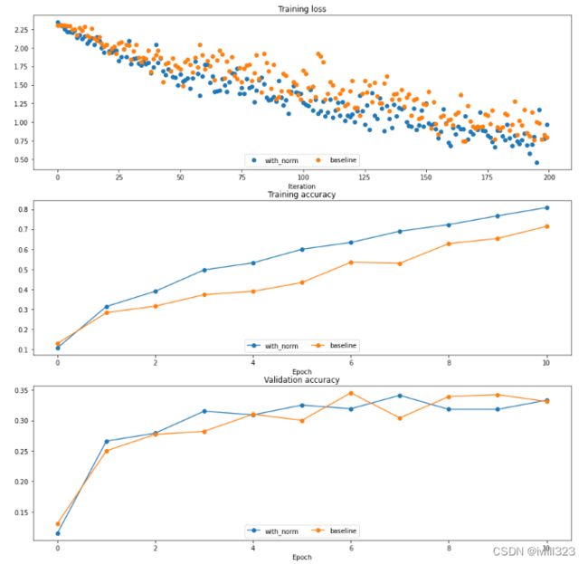
plt.subplot(3, 1, 1)
plot_training_history('Training loss','Iteration', solver, [bn_solver], \
                      lambda x: x.loss_history, bl_marker='o', bn_marker='o')
plt.subplot(3, 1, 2)
plot_training_history('Training accuracy','Epoch', solver, [bn_solver], \
                      lambda x: x.train_acc_history, bl_marker='-o', bn_marker='-o')
plt.subplot(3, 1, 3)
plot_training_history('Validation accuracy','Epoch', solver, [bn_solver], \
                      lambda x: x.val_acc_history, bl_marker='-o', bn_marker='-o')

plt.gcf().set_size_inches(15, 15)
plt.show()

You should find that using batch normalization helps the network to converge much faster.但是在测试结果上差别不大

 Batch Normalization 和初始化

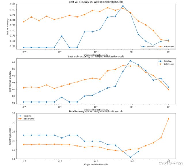
We will now run a small experiment to study the interaction of batch normalization and weight initialization.

The first cell will train eight-layer networks both with and without batch normalization using different scales for weight initialization. The second layer will plot training accuracy, validation set accuracy, and training loss as a function of the weight initialization scale.

np.random.seed(231)

# Try training a very deep net with batchnorm.
hidden_dims = [50, 50, 50, 50, 50, 50, 50]
num_train = 1000
small_data = {
  'X_train': data['X_train'][:num_train],
  'y_train': data['y_train'][:num_train],
  'X_val': data['X_val'],
  'y_val': data['y_val'],
}

bn_solvers_ws = {}
solvers_ws = {}
weight_scales = np.logspace(-4, 0, num=20)
for i, weight_scale in enumerate(weight_scales):
    print('Running weight scale %d / %d' % (i + 1, len(weight_scales)))
    bn_model = FullyConnectedNet(hidden_dims, weight_scale=weight_scale, normalization='batchnorm')
    model = FullyConnectedNet(hidden_dims, weight_scale=weight_scale, normalization=None)

    bn_solver = Solver(bn_model, small_data,
                  num_epochs=10, batch_size=50,
                  update_rule='adam',
                  optim_config={
                    'learning_rate': 1e-3,
                  },
                  verbose=False, print_every=200)
    bn_solver.train()
    bn_solvers_ws[weight_scale] = bn_solver

    solver = Solver(model, small_data,
                  num_epochs=10, batch_size=50,
                  update_rule='adam',
                  optim_config={
                    'learning_rate': 1e-3,
                  },
                  verbose=False, print_every=200)
    solver.train()
    solvers_ws[weight_scale] = solver

打印结果

# Plot results of weight scale experiment.
best_train_accs, bn_best_train_accs = [], []
best_val_accs, bn_best_val_accs = [], []
final_train_loss, bn_final_train_loss = [], []

for ws in weight_scales:
  best_train_accs.append(max(solvers_ws[ws].train_acc_history))
  bn_best_train_accs.append(max(bn_solvers_ws[ws].train_acc_history))
  
  best_val_accs.append(max(solvers_ws[ws].val_acc_history))
  bn_best_val_accs.append(max(bn_solvers_ws[ws].val_acc_history))
  
  final_train_loss.append(np.mean(solvers_ws[ws].loss_history[-100:]))
  bn_final_train_loss.append(np.mean(bn_solvers_ws[ws].loss_history[-100:]))
  
plt.subplot(3, 1, 1)
plt.title('Best val accuracy vs. weight initialization scale')
plt.xlabel('Weight initialization scale')
plt.ylabel('Best val accuracy')
plt.semilogx(weight_scales, best_val_accs, '-o', label='baseline')
plt.semilogx(weight_scales, bn_best_val_accs, '-o', label='batchnorm')
plt.legend(ncol=2, loc='lower right')

plt.subplot(3, 1, 2)
plt.title('Best train accuracy vs. weight initialization scale')
plt.xlabel('Weight initialization scale')
plt.ylabel('Best training accuracy')
plt.semilogx(weight_scales, best_train_accs, '-o', label='baseline')
plt.semilogx(weight_scales, bn_best_train_accs, '-o', label='batchnorm')
plt.legend()

plt.subplot(3, 1, 3)
plt.title('Final training loss vs. weight initialization scale')
plt.xlabel('Weight initialization scale')
plt.ylabel('Final training loss')
plt.semilogx(weight_scales, final_train_loss, '-o', label='baseline')
plt.semilogx(weight_scales, bn_final_train_loss, '-o', label='batchnorm')
plt.legend()
plt.gca().set_ylim(1.0, 3.5)

plt.gcf().set_size_inches(15, 15)
plt.show()

可以发现使用了Batch Normalization 之后，模型对初始化的鲁棒性更强了

 Batch Normalization 和 Batch Size

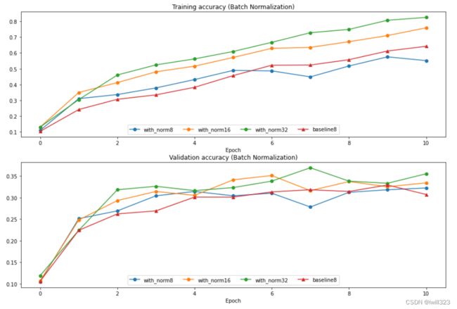
We will now run a small experiment to study the interaction of batch normalization and batch size.

The first cell will train 6-layer networks both with and without batch normalization using different batch sizes. The second layer will plot training accuracy and validation set accuracy over time.

def run_batchsize_experiments(normalization_mode):
    np.random.seed(231)
    
    # Try training a very deep net with batchnorm.
    hidden_dims = [100, 100, 100, 100, 100]
    num_train = 1000
    small_data = {
      'X_train': data['X_train'][:num_train],
      'y_train': data['y_train'][:num_train],
      'X_val': data['X_val'],
      'y_val': data['y_val'],
    }
    n_epochs=10
    weight_scale = 2e-2
    batch_sizes = [8,16,32]
    lr = 10**(-3.5)
    solver_bsize = batch_sizes[0]

    print('No normalization: batch size = ',solver_bsize)
    model = FullyConnectedNet(hidden_dims, weight_scale=weight_scale, normalization=None)
    solver = Solver(model, small_data,
                    num_epochs=n_epochs, batch_size=solver_bsize,
                    update_rule='adam',
                    optim_config={
                      'learning_rate': lr,
                    },
                    verbose=False)
    solver.train()
    
    bn_solvers = []
    for i in range(len(batch_sizes)):
        b_size=batch_sizes[i]
        print('Normalization: batch size = ',b_size)
        bn_model = FullyConnectedNet(hidden_dims, weight_scale=weight_scale, 
                                     normalization=normalization_mode)
        bn_solver = Solver(bn_model, small_data,
                        num_epochs=n_epochs, batch_size=b_size,
                        update_rule='adam',
                        optim_config={
                          'learning_rate': lr,
                        },
                        verbose=False)
        bn_solver.train()
        bn_solvers.append(bn_solver)
        
    return bn_solvers, solver, batch_sizes

bn_solvers_bsize, solver_bsize, batch_sizes = run_batchsize_experiments('batchnorm')

画出结果

plt.subplot(2, 1, 1)
plot_training_history('Training accuracy (Batch Normalization)','Epoch', solver_bsize, bn_solvers_bsize, \
                      lambda x: x.train_acc_history, bl_marker='-^', bn_marker='-o', labels=batch_sizes)
plt.subplot(2, 1, 2)
plot_training_history('Validation accuracy (Batch Normalization)','Epoch', solver_bsize, bn_solvers_bsize, \
                      lambda x: x.val_acc_history, bl_marker='-^', bn_marker='-o', labels=batch_sizes)

plt.gcf().set_size_inches(15, 10)
plt.show()

 batch size大，训练效果好。 batch size小的话可能还不如不用。batch size对测试结果影响不大

 Layer Normalization

Batch normalization has proved to be effective in making networks easier to train, but the dependency on batch size makes it less useful in complex networks which have a cap on the input batch size due to hardware limitations.

Layer Normalization：Instead of normalizing over the batch, we normalize over the features. In other words, when using Layer Normalization, each feature vector corresponding to a single datapoint is normalized based on the sum of all terms within that feature vector.

Ba, Jimmy Lei, Jamie Ryan Kiros, and Geoffrey E. Hinton. "Layer Normalization." stat 1050 (2016): 21.
For layer normalization, we do not keep track of the moving moments, and the testing phase is identical to the training phase, where the mean and variance are directly calculated per datapoint.

def layernorm_forward(x, gamma, beta, ln_param):
    """
    Note that in contrast to batch normalization, the behavior during train and test-time for
    layer normalization are identical, and we do not need to keep track of running averages
    of any sort.

    Input:
    - x: Data of shape (N, D)
    - gamma: Scale parameter of shape (D,)
    - beta: Shift paremeter of shape (D,)
    - ln_param: Dictionary with the following keys:
        - eps: Constant for numeric stability

    Returns a tuple of:
    - out: of shape (N, D)
    - cache: A tuple of values needed in the backward pass
    """
    out, cache = None, None
    eps = ln_param.get("eps", 1e-5)

    x_mean = np.mean(x, axis = 1, keepdims = True)
    x_var = np.var(x, axis = 1, keepdims = True) + eps
    x_std = np.sqrt(x_var)
    x_norm = (x - x_mean) / x_std
    out = x_norm *gamma + beta
    cache = (gamma, x, x_norm, x_mean, x_var)
    return out, cache

def layernorm_backward(dout, cache):
    gamma,x, x_norm,  mean, var = cache
    std = np.sqrt(var)
    dgamma = np.sum(dout * x_norm, axis = 0)
    dbeta = np.sum(dout, axis = 0)

    D = 1.0 * x.shape[1]   
    dfdu = dout * gamma
    dfdv = np.sum(dfdu * (x - mean) * -0.5 * var ** -1.5, axis = 1)
    dfdw = np.sum(dfdu * -1 / std, axis = 1) + dfdv * np.sum(-2/D * (x - mean), axis = 1)
    # dfdv 和 dfdw.shape的形状都是（N,） dfdv.reshape(-1, 1)形状是（N，1）
    dx = dfdu / std + dfdv.reshape(-1, 1) * 2/D * (x - mean) + dfdw.reshape(-1, 1) / D
    return dx, dgamma, dbeta

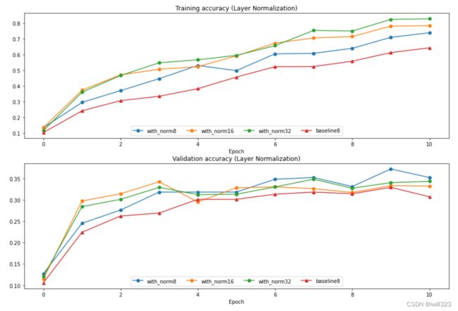
Layer Normalization 和 Batch Size

ln_solvers_bsize, solver_bsize, batch_sizes = run_batchsize_experiments('layernorm')

plt.subplot(2, 1, 1)
plot_training_history('Training accuracy (Layer Normalization)','Epoch', solver_bsize, ln_solvers_bsize, \
                      lambda x: x.train_acc_history, bl_marker='-^', bn_marker='-o', labels=batch_sizes)
plt.subplot(2, 1, 2)
plot_training_history('Validation accuracy (Layer Normalization)','Epoch', solver_bsize, ln_solvers_bsize, \
                      lambda x: x.val_acc_history, bl_marker='-^', bn_marker='-o', labels=batch_sizes)

plt.gcf().set_size_inches(15, 10)
plt.show()

Compared to the previous experiment, you should see a markedly smaller influence of batch size on the training history!

卷积层的batch norm--spatial batchnorm

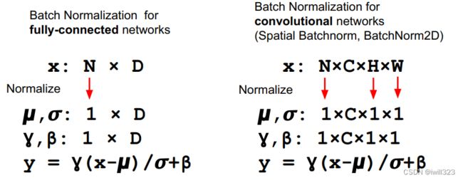
If the feature map was produced using convolutions, then we expect every feature channel's statistics e.g. mean, variance to be relatively consistent both between different images, and different locations within the same image -- after all, every feature channel is produced by the same convolutional filter! Therefore, spatial batch normalization computes a mean and variance for each of the C feature channels by computing statistics over the minibatch dimension N as well the spatial dimensions H and W.

 正向传播

def spatial_batchnorm_forward(x, gamma, beta, bn_param):
    """
    Inputs:
    - x: Input data of shape (N, C, H, W)
    - gamma: Scale parameter, of shape (C,)
    - beta: Shift parameter, of shape (C,)
    - bn_param: Dictionary with the following keys:
      - mode: 'train' or 'test'; required
      - eps: Constant for numeric stability
      - momentum: Constant for running mean / variance. momentum=0 means that
        old information is discarded completely at every time step, while
        momentum=1 means that new information is never incorporated. The
        default of momentum=0.9 should work well in most situations.
      - running_mean: Array of shape (D,) giving running mean of features
      - running_var Array of shape (D,) giving running variance of features

    Returns a tuple of:
    - out: Output data, of shape (N, C, H, W)
    - cache: Values needed for the backward pass
    """
    out, cache = None, None
    N, C, H, W = x.shape
    x_trans = x.transpose(0,2,3,1).reshape(N*H*W, C)  # 对每一个C进行归一化
    out1, cache = batchnorm_forward(x_trans, gamma, beta, bn_param)
    out = out1.reshape(N, H, W, C).transpose(0,3,1,2)  

    return out, cache

反向传播

def spatial_batchnorm_backward(dout, cache):
    """Computes the backward pass for spatial batch normalization.

    Inputs:
    - dout: Upstream derivatives, of shape (N, C, H, W)
    - cache: Values from the forward pass

    Returns a tuple of:
    - dx: Gradient with respect to inputs, of shape (N, C, H, W)
    - dgamma: Gradient with respect to scale parameter, of shape (C,)
    - dbeta: Gradient with respect to shift parameter, of shape (C,)
    """
    N, C, H, W = dout.shape
    dout_trans = dout.transpose(0,2,3,1).reshape(N*H*W, C)
    dx, dgamma, dbeta = batchnorm_backward_alt(dout_trans, cache)
    dx = dx.reshape(N, H, W, C).transpose(0,3,1,2)

    return dx, dgamma, dbeta

Spatial Group Normalization

as the authors of [2] observed, Layer Normalization does not perform as well as Batch Normalization when used with Convolutional Layers:

With fully connected layers, all the hidden units in a layer tend to make similar contributions to the final prediction, and re-centering and rescaling the summed inputs to a layer works well. However, the assumption of similar contributions is no longer true for convolutional neural networks. The large number of the hidden units whose receptive fields lie near the boundary of the image are rarely turned on and thus have very different statistics from the rest of the hidden units within the same layer.

The authors of [3] propose an intermediary technique. In contrast to Layer Normalization, where you normalize over the entire feature per-datapoint, they suggest a consistent splitting of each per-datapoint feature into G groups and a per-group per-datapoint normalization instead.

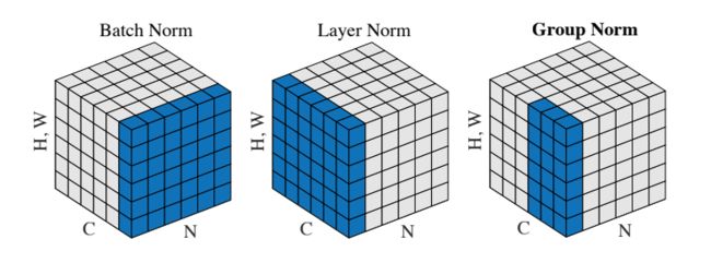
Even though an assumption of equal contribution is still being made within each group, the authors hypothesize that this is not as problematic, as innate grouping arises within features for visual recognition. One example they use to illustrate this is that many high-performance handcrafted features in traditional computer vision have terms that are explicitly grouped together. Take for example Histogram of Oriented Gradients [4] -- after computing histograms per spatially local block, each per-block histogram is normalized before being concatenated together to form the final feature vector.

[2] Ba, Jimmy Lei, Jamie Ryan Kiros, and Geoffrey E. Hinton. "Layer Normalization." stat 1050 (2016): 21.

[3] Wu, Yuxin, and Kaiming He. "Group Normalization." arXiv preprint arXiv:1803.08494 (2018).

[4] N. Dalal and B. Triggs. Histograms of oriented gradients for human detection. In Computer Vision and Pattern Recognition (CVPR), 2005.

正向传播

def spatial_groupnorm_forward(x, gamma, beta, G, gn_param):
    """
    In contrast to layer normalization, group normalization splits each entry in the data into G
    contiguous pieces, which it then normalizes independently. Per-feature shifting and scaling
    are then applied to the data, in a manner identical to that of batch normalization and layer
    normalization.

    Inputs:
    - x: Input data of shape (N, C, H, W)
    - gamma: Scale parameter, of shape (1, C, 1, 1)
    - beta: Shift parameter, of shape (1, C, 1, 1)
    - G: Integer mumber of groups to split into, should be a divisor of C
    - gn_param: Dictionary with the following keys:
      - eps: Constant for numeric stability

    Returns a tuple of:
    - out: Output data, of shape (N, C, H, W)
    - cache: Values needed for the backward pass
    """
    out, cache = None, None
    eps = gn_param.get("eps", 1e-5)

    N, C, H, W = x.shape
    x_trans = x.reshape(N, G, C//G, H, W)
    mean = np.mean(x_trans, axis = (2,3,4), keepdims = True)
    var = np.var(x_trans, axis = (2,3,4), keepdims = True) + eps
    std = np.sqrt(var)
    x_norm = (x_trans - mean) / std
    x_norm = x_norm.reshape(x.shape)
    out = x_norm * gamma + beta

    cache = (x, x_norm, gamma, mean, var, std, G)

    return out, cache

 反向传播

def spatial_groupnorm_backward(dout, cache):
    """

    Inputs:
    - dout: Upstream derivatives, of shape (N, C, H, W)
    - cache: Values from the forward pass

    Returns a tuple of:
    - dx: Gradient with respect to inputs, of shape (N, C, H, W)
    - dgamma: Gradient with respect to scale parameter, of shape (1, C, 1, 1)
    - dbeta: Gradient with respect to shift parameter, of shape (1, C, 1, 1)
    """
    dx, dgamma, dbeta = None, None, None

    x, x_norm, gamma, mean, var, std, G = cache
    N, C, H, W = x.shape
    dgamma = np.sum(dout * x_norm, axis = (0,2,3))[None, :, None, None]
    dbeta = np.sum(dout, axis = (0,2,3))[None, :, None, None]
    x_trans = x.reshape(N, G, C//G, H, W)

    M = C // G * H * W
    dfdu = (dout * gamma).reshape(N, G, C//G, H, W)
    dfdv = np.sum(dfdu * (x_trans - mean) * -0.5 * var ** -1.5, axis = (2,3,4))
    dfdw = np.sum(dfdu * -1 / std, axis = (2,3,4)) + dfdv * np.sum(-2/N * (x_trans - mean), axis = (2,3,4))
    dx = dfdu / std + dfdv.reshape(N, G, 1, 1, 1) * 2/M * (x_trans - mean) + dfdw.reshape(N, G, 1, 1, 1) / M
    dx = dx.reshape(x.shape)
    return dx, dgamma, dbeta

dropout

正向传播

def dropout_forward(x, dropout_param):
    """

    Note that this is different from the vanilla version of dropout.
    Here, p is the probability of keeping a neuron output, as opposed to
    the probability of dropping a neuron output.

    Inputs:
    - x: Input data, of any shape
    - dropout_param: A dictionary with the following keys:
      - p: Dropout parameter. We keep each neuron output with probability p.
      - mode: 'test' or 'train'. If the mode is train, then perform dropout;
        if the mode is test, then just return the input.

    Outputs:
    - out: Array of the same shape as x.
    - cache: tuple (dropout_param, mask). In training mode, mask is the dropout
      mask that was used to multiply the input; in test mode, mask is None.
    """
    p, mode = dropout_param["p"], dropout_param["mode"]
    if "seed" in dropout_param:
        np.random.seed(dropout_param["seed"])

    mask = None
    out = None

    if mode == "train":
        mask = (np.random.rand(*x.shape) < p )/ p # 这地方不能用np.random.randn()
        out = x * mask 
        
    elif mode == "test":
        out = x

    cache = (dropout_param, mask)
    out = out.astype(x.dtype, copy=False)

    return out, cache

反向传播

def dropout_backward(dout, cache):
    """

    Inputs:
    - dout: Upstream derivatives, of any shape
    - cache: (dropout_param, mask) from dropout_forward.
    """
    dropout_param, mask = cache
    mode = dropout_param["mode"]

    dx = None
    if mode == "train":        
        dx = dout * mask
    elif mode == "test":
        dx = dout
    return dx

Regularization Experiment

As an experiment, we will train a pair of two-layer networks on 500 training examples: one will use no dropout, and one will use a keep probability of 0.25. We will then visualize the training and validation accuracies of the two networks over time.

# Train two identical nets, one with dropout and one without.
np.random.seed(231)
num_train = 500
small_data = {
    'X_train': data['X_train'][:num_train],
    'y_train': data['y_train'][:num_train],
    'X_val': data['X_val'],
    'y_val': data['y_val'],
}

solvers = {}
dropout_choices = [1, 0.25]
for dropout_keep_ratio in dropout_choices:
    model = FullyConnectedNet(
        [500],
        dropout_keep_ratio=dropout_keep_ratio
    )
    print(dropout_keep_ratio)

    solver = Solver(
        model,
        small_data,
        num_epochs=25,
        batch_size=100,
        update_rule='adam',
        optim_config={'learning_rate': 5e-4,},
        verbose=True,
        print_every=100
    )
    solver.train()
    solvers[dropout_keep_ratio] = solver
    print()

显示结果

# Plot train and validation accuracies of the two models.
train_accs = []
val_accs = []
for dropout_keep_ratio in dropout_choices:
    solver = solvers[dropout_keep_ratio]
    train_accs.append(solver.train_acc_history[-1])
    val_accs.append(solver.val_acc_history[-1])

plt.subplot(3, 1, 1)
for dropout_keep_ratio in dropout_choices:
    plt.plot(
        solvers[dropout_keep_ratio].train_acc_history, 'o', label='%.2f dropout_keep_ratio' % dropout_keep_ratio)
plt.title('Train accuracy')
plt.xlabel('Epoch')
plt.ylabel('Accuracy')
plt.legend(ncol=2, loc='lower right')
  
plt.subplot(3, 1, 2)
for dropout_keep_ratio in dropout_choices:
    plt.plot(
        solvers[dropout_keep_ratio].val_acc_history, 'o', label='%.2f dropout_keep_ratio' % dropout_keep_ratio)
plt.title('Val accuracy')
plt.xlabel('Epoch')
plt.ylabel('Accuracy')
plt.legend(ncol=2, loc='lower right')

plt.gcf().set_size_inches(15, 15)
plt.show()

 Solver和网络

solver

from __future__ import print_function, division
from future import standard_library
from cs231n import optim
 
standard_library.install_aliases()
import os
import pickle as pickle
 
class Solver(object):  
 
    def __init__(self, model, data, **kwargs):
        self.model = model
        self.X_train = data['X_train']
        self.y_train = data["y_train"]
        self.X_val = data["X_val"]
        self.y_val = data["y_val"]
 
        # Unpack keyword arguments
        self.update_rule = kwargs.pop("update_rule", "sgd")
        self.optim_config = kwargs.pop("optim_config", {})
        self.lr_decay = kwargs.pop("lr_decay", 1.0)
        self.batch_size = kwargs.pop("batch_size", 100)
        self.num_epochs = kwargs.pop("num_epochs", 10)
        self.num_train_samples = kwargs.pop("num_train_samples", 1000)
        self.num_val_samples = kwargs.pop("num_val_samples", None)
 
        self.checkpoint_name = kwargs.pop("checkpoint_name", None)
        self.print_every = kwargs.pop("print_every", 10)
        self.verbose = kwargs.pop("verbose", True)
 
        # Throw an error if there are extra keyword arguments
        if len(kwargs) > 0:
            extra = ", ".join('"%s"' % k for k in list(kwargs.keys()))
            raise ValueError("Unrecognized arguments %s" % extra)
 
        # Make sure the update rule exists, then replace the string name with the actual function
        if not hasattr(optim, self.update_rule):
            raise ValueError('Invalid update_rule "%s"' % self.update_rule)
        self.update_rule = getattr(optim, self.update_rule)
        # hasattr() 函数用于判断对象是否包含对应的属性。 在optim包中找对应的update_rule 
        self._reset()
 
    def _reset(self):
        """
        Set up some book-keeping variables for optimization. Don't call this manually.
        """
        # Set up some variables for book-keeping
        self.epoch = 0
        self.best_val_acc = 0
        self.best_params = {}
        self.loss_history = []
        self.train_acc_history = []
        self.val_acc_history = []
 
        # Make a deep copy of the optim_config for each parameter
        self.optim_configs = {}
        for p in self.model.params:  # model.params是一个字典
            d = {k: v for k, v in self.optim_config.items()} # optim_config是字典
            self.optim_configs[p] = d   # optim_configs每一个元素岂不是一样？
 
    def _step(self):
        # Make a minibatch of training data
        num_train = self.X_train.shape[0]
        batch_mask = np.random.choice(num_train, self.batch_size)
        X_batch = self.X_train[batch_mask]
        y_batch = self.y_train[batch_mask]
 
        # Compute loss and gradient
        loss, grads = self.model.loss(X_batch, y_batch)
        self.loss_history.append(loss)
 
        # Perform a parameter update
        for p, w in self.model.params.items():  # model.params是一个字典
            dw = grads[p]  # dw只是一个名字，实际上可以是任何参数
            config = self.optim_configs[p]  # 比如learning rate
            next_w, next_config = self.update_rule(w, dw, config)
            self.model.params[p] = next_w
            self.optim_configs[p] = next_config
 
    def _save_checkpoint(self):
        if self.checkpoint_name is None:
            return
        checkpoint = {
            "model": self.model,
            "update_rule": self.update_rule,
            "lr_decay": self.lr_decay,
            "optim_config": self.optim_config,
            "batch_size": self.batch_size,
            "num_train_samples": self.num_train_samples,
            "num_val_samples": self.num_val_samples,
            "epoch": self.epoch,
            "loss_history": self.loss_history,
            "train_acc_history": self.train_acc_history,
            "val_acc_history": self.val_acc_history,
        }
        filename = "%s_epoch_%d.pkl" % (self.checkpoint_name, self.epoch)
        if self.verbose:
            print('Saving checkpoint to "%s"' % filename)
        with open(filename, "wb") as f:
            pickle.dump(checkpoint, f)
 
    def check_accuracy(self, X, y, num_samples=None, batch_size=100):
        """
        Check accuracy of the model on the provided data.
        Inputs:
        - X: Array of data, of shape (N, d_1, ..., d_k)
        - y: Array of labels, of shape (N,)
        - num_samples: If not None, subsample the data and only test the model
          on num_samples datapoints.
        - batch_size: Split X and y into batches of this size to avoid using
          too much memory.
        Returns:
        - acc: Scalar giving the fraction of instances that were correctly
          classified by the model.
        """
 
        # Maybe subsample the data
        N = X.shape[0]
        if num_samples is not None and N > num_samples:
            mask = np.random.choice(N, num_samples)
            N = num_samples
            X = X[mask]
            y = y[mask]
 
        # Compute predictions in batches
        num_batches = N // batch_size
        if N % batch_size != 0:
            num_batches += 1
        y_pred = []
        for i in range(num_batches):
            start = i * batch_size
            end = (i + 1) * batch_size
            scores = self.model.loss(X[start:end])  
            # model.loss中y==none返回的是score
            y_pred.append(np.argmax(scores, axis=1))
        y_pred = np.hstack(y_pred)
        acc = np.mean(y_pred == y)
 
        return acc
 
    def train(self):
        """
        Run optimization to train the model.
        """
        num_train = self.X_train.shape[0]
        iterations_per_epoch = max(num_train // self.batch_size, 1)
        num_iterations = self.num_epochs * iterations_per_epoch
 
        for t in range(num_iterations):
            self._step()
 
            # Maybe print training loss
            if self.verbose and t % self.print_every == 0:
                print(
                    "(Iteration %d / %d) loss: %f"
                    % (t + 1, num_iterations, self.loss_history[-1])
                )
 
            # At the end of every epoch, increment the epoch counter and decay
            # the learning rate.
            epoch_end = (t + 1) % iterations_per_epoch == 0
            if epoch_end:
                self.epoch += 1
                for k in self.optim_configs:
                    self.optim_configs[k]["learning_rate"] *= self.lr_decay
 
            # Check train and val accuracy on the first iteration, the last
            # iteration, and at the end of each epoch.
            first_it = t == 0
            last_it = t == num_iterations - 1
            if first_it or last_it or epoch_end:
                train_acc = self.check_accuracy(
                    self.X_train, self.y_train, num_samples=self.num_train_samples
                )
                val_acc = self.check_accuracy(
                    self.X_val, self.y_val, num_samples=self.num_val_samples
                )
                self.train_acc_history.append(train_acc)
                self.val_acc_history.append(val_acc)
                self._save_checkpoint()
 
                if self.verbose:
                    print(
                        "(Epoch %d / %d) train acc: %f; val_acc: %f"
                        % (self.epoch, self.num_epochs, train_acc, val_acc)
                    )
 
                # Keep track of the best model
                if val_acc > self.best_val_acc:
                    self.best_val_acc = val_acc
                    self.best_params = {}
                    for k, v in self.model.params.items():
                        self.best_params[k] = v.copy()
 
        # At the end of training swap the best params into the model
        self.model.params = self.best_params

 网络

import numpy as np

# from cs231n.layers import *
# from cs231n.layer_utils import *


class FullyConnectedNet(object):
    def __init__(
        self,
        hidden_dims,
        input_dim=3 * 32 * 32,
        num_classes=10,
        dropout_keep_ratio=1,
        normalization=None,
        reg=0.0,
        weight_scale=1e-2,
        dtype=np.float32,
        seed=None,
    ):
        
        self.normalization = normalization
        self.use_dropout = dropout_keep_ratio != 1
        self.reg = reg
        self.num_layers = 1 + len(hidden_dims)
        self.dtype = dtype
        self.params = {}

        dims = np.hstack((input_dim, hidden_dims, num_classes))
        for i in range(self.num_layers): 
            W = np.random.randn(dims[i], dims[i+1]) * weight_scale            
            b = np.zeros(dims[i+1])
            self.params['W' + str(i+1)] = W
            self.params['b' + str(i+1)] = b
            
        if self.normalization != None:
            for i in range(self.num_layers - 1):  # 最后一层的输出不用做batchnorm
                self.params['gamma' + str(i+1)] = np.ones(dims[i+1])
                self.params['beta' + str(i+1)] = np.zeros(dims[i+1])


        # When using dropout we need to pass a dropout_param dictionary to each
        # dropout layer so that the layer knows the dropout probability and the mode
        # (train / test). You can pass the same dropout_param to each dropout layer.
        self.dropout_param = {}
        if self.use_dropout:
            self.dropout_param = {"mode": "train", "p": dropout_keep_ratio}
            if seed is not None:
                self.dropout_param["seed"] = seed

        # With batch normalization we need to keep track of running means and
        # variances, so we need to pass a special bn_param object to each batch
        # normalization layer. You should pass self.bn_params[0] to the forward pass
        # of the first batch normalization layer, self.bn_params[1] to the forward
        # pass of the second batch normalization layer, etc.
        self.bn_params = []
        if self.normalization == "batchnorm":
            self.bn_params = [{"mode": "train"} for i in range(self.num_layers - 1)]
        if self.normalization == "layernorm":
            self.bn_params = [{} for i in range(self.num_layers - 1)]

        # Cast all parameters to the correct datatype.
        for k, v in self.params.items():
            self.params[k] = v.astype(dtype)

    def loss(self, X, y=None):        
        X = X.astype(self.dtype)
        mode = "test" if y is None else "train"

        # Set train/test mode for batchnorm params and dropout param since they
        # behave differently during training and testing.
        if self.use_dropout:
            self.dropout_param["mode"] = mode
        if self.normalization == "batchnorm":
            for bn_param in self.bn_params:
                bn_param["mode"] = mode  # bn_param是字典
        scores = None    

        
        # For a network with L layers, the architecture will be #
        #{affine - [batch/layer norm] - relu - [dropout]} x (L - 1)-affine -softmax#

        caches = []
        drop_caches = []
        x = X
        drop_cache = None
        gamma, beta, bn_params = None, None, None
        
        for i in range(self.num_layers - 1):
            W = self.params['W' + str(i+1)]
            b = self.params['b' + str(i+1)]
            if self.normalization != None:                
                gamma = self.params['gamma'+ str(i+1)]
                beta = self.params['beta' + str(i+1)]
                bn_params = self.bn_params[i]
            
            # print(b.shape)
            #print(bn_params)
            x, cache = affine_norm_relu_forward(x, W, b, gamma, beta, bn_params, 
                                                self.normalization, self.use_dropout, 
                                                self.dropout_param)
            if self.use_dropout:
                x, drop_cache = dropout_forward(x, self.dropout_param)
     
            caches.append(cache)
            drop_caches.append(drop_cache)

        W = self.params['W' + str(self.num_layers)]
        b = self.params['b' + str(self.num_layers)]
        scores, cache = affine_forward(x, W, b)
        caches.append(cache)
        
        # If test mode return early.
        if mode == "test":
            return scores

        loss, grads = 0.0, {}

        loss, softmax_grad = softmax_loss(scores, y)
        for i in range(self.num_layers):
            W = self.params['W'+str(i+1)]
            loss += 0.5 * self.reg *(W ** 2).sum()
            
        dout, dw, db = affine_backward(softmax_grad, caches[self.num_layers - 1])
        grads['W' + str(self.num_layers)] = dw + self.reg * self.params['W'+str(self.num_layers)]
        grads['b' + str(self.num_layers)] = db

        for i in range(self.num_layers - 2, -1, -1):
            if self.use_dropout:
                dout = dropout_backward(dout, drop_caches[i]) 
            # 倒数第二层，drop_cache和caches对应的元素下标是num_layers - 2
            dx, dw, db, dgamma, dbeta = affine_norm_relu_backward(dout, caches[i], self.normalization, self.use_dropout)
            grads['W' + str(i+1)] = dw + self.reg * self.params['W'+str(i+1)]
            grads['b' + str(i + 1)] = db
            if self.normalization != None:
                grads['gamma'+str(i+1)] = dgamma
                grads['beta' +str(i+1)] = dbeta
            dout = dx
            
        return loss, grads

网络用到的辅助函数（各层）

#  layers.py

def affine_forward(x, w, b):    
    x_vector = x.reshape(x.shape[0], -1) 
    out = x_vector.dot(w) + b 
    # 上面第一项形状是(N, M)，b的形状是(M,)，广播机制要求x_vector的最后一维和b一致
    cache = (x, w, b)
    return out, cache


def affine_backward(dout, cache):
    x, w, b = cache
    dx = dout.dot(w.T).reshape(x.shape) # (N, M) @ (M, D)
    x_vector = x.reshape(x.shape[0], -1)
    dw = x_vector.T.dot(dout)  # (D, N) @ (N, M)    
    # db = np.dot(dout.T, np.ones(x.shape[0])) # dout.T：(M, N) 相当于每一行求和
    db = dout.sum(axis=0) # 这么写也对   为什么是求和不是求平均？
    return dx, dw, db

def relu_forward(x):
    out = np.maximum(0,x)
    cache = x
    return out, cache


def relu_backward(dout, cache):
    dx, x = None, cache
    dx = x
    dx[dx < 0] = 0  # x是否会被改变？
    dx[dx > 0] = 1
    dx *= dout
    return dx


def affine_norm_relu_forward(x, W, b, gamma, beta, bn_params, normalization,
                            use_dropout, dropout_param):    
    out, fc_cache = affine_forward(x, W, b)
    norm_cache, drop_cache = None, None
    if normalization == 'batchnorm':
        out, norm_cache = batchnorm_forward(out, gamma, beta, bn_params)
    elif normalization == 'layernorm':
        out, norm_cache = layernorm_forward(out, gamma, beta, bn_params)
    out, relu_cache = relu_forward(out)
    if use_dropout:
        out, drop_cache = dropout_forward(out, dropout_param)
        
    cache = (fc_cache, norm_cache, relu_cache, drop_cache)
    return out, cache

def affine_norm_relu_backward(dout, cache, normalization, use_dropout):
    fc_cache, norm_cache, relu_cache, drop_cache = cache
    if use_dropout:
        dout = dropout_backward(dout, drop_cache)
    dout = relu_backward(dout, relu_cache)
    dgamma, dbeta = None, None # 必须要有这一行，因为return总要返回值
    if normalization == 'batchnorm':
        dout, dgamma, dbeta = batchnorm_backward_alt(dout, norm_cache)
    elif normalization == 'layernorm':
        dout, dgamma, dbeta = layernorm_backward(dout, norm_cache)
    dx, dw, db = affine_backward(dout, fc_cache)
    
    return dx, dw, db, dgamma, dbeta

损失函数

def softmax_loss(x, y):    
    loss, dx = None, None

    num_train = x.shape[0]
    scores = x - np.max(x, axis = 1).reshape(-1, 1)
    normalized_scores = np.exp(scores) / np.sum(np.exp(scores), axis = 1).reshape(-1,1)
    loss = -np.sum(np.log(normalized_scores[np.arange(num_train), y]))
    loss /= num_train

    normalized_scores[np.arange(num_train), y] -= 1
    dx = normalized_scores / num_train
    return (loss, dx)