sklearn学习01——LinearRegression / LogisticRegression

---

前言

在学习了机器学习（周志华）的一系列的模型和学习算法之后，我们也需要使用python实际操作，实现它的效果，进而深入理解这些模型的原理。本篇讲解 几种线性回归 的sklearn实现。

---

一、一/多元线性回归

1.1、数据生成

仅为了更加方便直观的理解机器学习算法，这里使用人工生成的简单数据。生成数据的思路是：设定一个二维的函数（维度高了没办法在平面上画出来），根据这个函数生成一些离散的数据点，对每个数据点我们可以适当的加一点波动，也就是噪声。代码如下：

import numpy as np
import matplotlib.pyplot as plt 

def true_fun(X): # 这是我们设定的真实函数，我们的模型越接近它越好
    return 1.5*X + 0.2

np.random.seed(0) # 设置随机种子
n_samples = 30 # 设置采样数据点的个数

'''生成随机数据作为训练集，并且加一些噪声'''
X_train = np.sort(np.random.rand(n_samples)) 
y_train = (true_fun(X_train) + np.random.randn(n_samples) * 0.05).reshape(n_samples,1)

30个样本，每个样本都只有一个特征（因为是一维的）。

注意：噪声是按照正态分布随机生成的30个数，附加到每个样本的 y 上，因此 y 也是符合正态分布的了。

1.2、得到模型

第一步生成好了数据，即有了训练集。接下来可以定义我们的算法模型，因为sklearn库中有类LinearRegression，所以直接调用它作为我们的线性模型即可。我们要做的就是：将训练集放入该LinearRegression模型中，然后等待它调用自己内部的方法求得最优解。代码如下：

from sklearn.linear_model import LinearRegression # 导入线性回归模型
model = LinearRegression() # 定义模型
model.fit(X_train[:,np.newaxis], y_train) # 训练模型
print("输出参数w：",model.coef_) # 输出模型参数w
print("输出参数b：",model.intercept_) # 输出参数b

输出参数w： [[1.4474774]]
输出参数b： [0.22557542]

1.3、模型测试和比较

第二步我们根据训练集和 sklearn 库中的模型算法得到一组解，写成方程形式为：y = 1.4474774 * x + 0.22557542，而真实的函数为：y = 1.5*x + 0.2，相比来说还是非常接近的。下面使用python代码将训练集（30个样本点）、我们学得的模型、真实模型都可视化出来：

X_test = np.linspace(0, 1, 100)
plt.plot(X_test, model.predict(X_test[:, np.newaxis]), label="Model")
plt.plot(X_test, true_fun(X_test), label="True function")
plt.scatter(X_train,y_train) # 画出训练集的点
plt.legend(loc="best")
plt.show()

1.4、多元线性回归

多元的线性回归，思路与一元是一样的。使用sklearn库来实现的话，我们只需要准备一组 多元的训练集 即可，依旧调用 内部的LinearRegression类 实现模型的训练，代码如下：

from sklearn.linear_model import LinearRegression

X_train = [[1,1,1],[1,1,2],[1,2,1]] # 以三元为例
y_train = [[6],[9],[8]]
 
model = LinearRegression()
model.fit(X_train, y_train)
print("输出参数w:",model.coef_) # 输出参数w1,w2,w3
print("输出参数b:",model.intercept_) # 输出参数b
test_X = [[1,3,5]]
pred_y = model.predict(test_X)
print("预测结果:",pred_y)

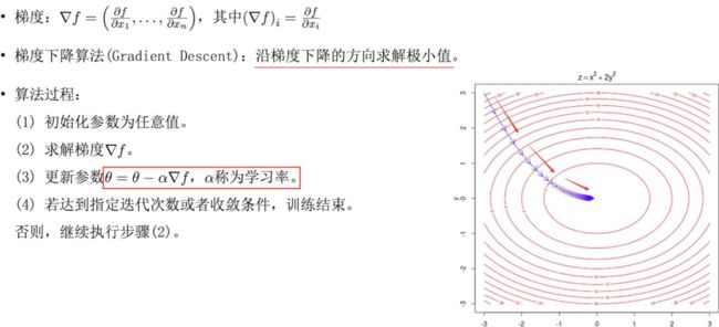
1.5、训练一元线性模型常用方法——梯度下降法

梯度下降法大致流程如下图：

首先先假定我们的线性模型为：
那么损失函数为：

要求损失函数最小值，我们对其求梯度：

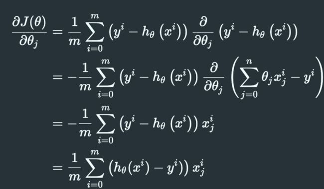
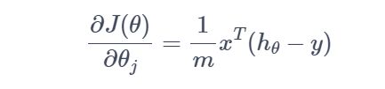
上述梯度使用矩阵形式表示：

在使用梯度下降算法更新我们线性模型的参数时，先初始化这些参数为全 1，然后按照梯度下降的方向更新所有的参数（批量梯度下降），达到迭代次数或者达到精度即可停止更新。代码如下：

import numpy as np
import matplotlib.pyplot as plt

# 梯度下降方法 实现一元线性回归模型
def true_fun(X):
    return 1.5 * X + 0.2


np.random.seed(0)  # 随机种子
n_samples = 30
'''生成随机数据作为训练集'''
X_train = np.sort(np.random.rand(n_samples))
y_train = (true_fun(X_train) + np.random.randn(n_samples) * 0.05).reshape(n_samples, 1)

# 添加一维数据
data_X = []
for x in X_train:
    data_X.append([1, x])

print(data_X)
data_X = np.array((data_X))
print(data_X)

m,p = np.shape(data_X) # m, 数据量 p: 特征数
max_iter = 1000 # 迭代数
weights = np.ones((p,1))   # 初始权重：设置为 1
print(weights)
alpha = 0.1 # 学习率
for i in range(0,max_iter):
    error = np.dot(data_X,weights)- y_train
    gradient = data_X.transpose().dot(error)/m
    weights = weights - alpha * gradient
print("输出参数w:",weights[1:][0]) # 输出模型参数w
print("输出参数b:",weights[0]) # 输出参数b

X_test = np.linspace(0, 1, 100)
plt.plot(X_test, X_test*weights[1][0]+weights[0][0], label="Model")
plt.plot(X_test, true_fun(X_test), label="True function")
plt.scatter(X_train,y_train) # 画出训练集的点
plt.legend(loc="best")
plt.show()

输出参数w: 1.4454389990357697
输出参数b: 0.2268326207539249

二、多项式线性回归

• 训练集
  用来训练模型内参数的数据集
• 验证集
  用于在训练过程中检验模型的状态，收敛情况，通常用于调整超参数，根据几组模型验证集上的表现决定哪组超参数拥有最好的性能。
  同时验证集在训练过程中还可以用来监控模型是否发生过拟合，一般来说验证集表现稳定后，若继续训练，训练集表现还会继续上升，但是验证集会出现不升反降的情况，这样一般就发生了过拟合。所以验证集也用来判断何时停止训练
• 测试集
  测试集用来评价模型泛化能力，即使用训练集调整了参数，之前模型使用验证集确定了超参数，最后使用一个不同的数据集来检查模型。

这里我们使用 交叉验证方法来获得多组的 训练集/测试集，求得每组的模型评估（回归的评估度量手段一般为均方误差）然后求平均，作为评估此模型的标准。

多项式回归代码如下（这里尝试了三个最高次 1、4、15）：

import numpy as np
import matplotlib.pyplot as plt
from sklearn.pipeline import Pipeline
from sklearn.preprocessing import PolynomialFeatures
from sklearn.linear_model import LinearRegression
from sklearn.model_selection import cross_val_score

def true_fun(X):
    return np.cos(1.5 * np.pi * X)
np.random.seed(0)

n_samples = 30
degrees = [1, 4, 15] # 多项式最高次

X = np.sort(np.random.rand(n_samples)) 
y = true_fun(X) + np.random.randn(n_samples) * 0.1

plt.figure(figsize=(14, 5))
for i in range(len(degrees)):
    ax = plt.subplot(1, len(degrees), i + 1)
    plt.setp(ax, xticks=(), yticks=())

    polynomial_features = PolynomialFeatures(degree=degrees[i],
                                             include_bias=False)
    linear_regression = LinearRegression()
    pipeline = Pipeline([("polynomial_features", polynomial_features),
                         ("linear_regression", linear_regression)]) # 使用pipline串联模型
    pipeline.fit(X[:, np.newaxis], y)

    # 使用交叉验证
    scores = cross_val_score(pipeline, X[:, np.newaxis], y,
                             scoring="neg_mean_squared_error", cv=10)
    X_test = np.linspace(0, 1, 100)
    plt.plot(X_test, pipeline.predict(X_test[:, np.newaxis]), label="Model")
    plt.plot(X_test, true_fun(X_test), label="True function")
    plt.scatter(X, y, edgecolor='b', s=20, label="Samples")
    plt.xlabel("x")
    plt.ylabel("y")
    plt.xlim((0, 1))
    plt.ylim((-2, 2))
    plt.legend(loc="best")
    plt.title("Degree {}\nMSE = {:.2e}(+/- {:.2e})".format(
        degrees[i], -scores.mean(), scores.std()))
plt.show()

三、逻辑（Logistic）回归

3.1、损失函数

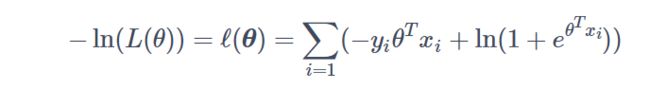
我们知道，在线性模型上套一个Sigmoid函数就成了对数几率回归（具体参考西瓜书），假设此模型为：


再参考西瓜书得到其损失函数，这里直接写出来：

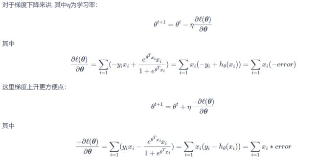
3.2、梯度下降法

3.3、代码实现

import sys
from pathlib import Path
curr_path = str(Path().absolute())
parent_path = str(Path().absolute().parent)
sys.path.append(parent_path) # add current terminal path to sys.path

import numpy as np
from Mnist.load_data import load_local_mnist

(x_train, y_train), (x_test, y_test) = load_local_mnist(one_hot=False)

# print(np.shape(x_train),np.shape(y_train))

ones_col=[[1] for i in range(len(x_train))] # 生成全为1的二维嵌套列表，即[[1],[1],...,[1]]
x_train_modified=np.append(x_train,ones_col,axis=1)
ones_col=[[1] for i in range(len(x_test))]
x_test_modified=np.append(x_test,ones_col,axis=1)

# print(np.shape(x_train_modified))

# Mnsit有0-9十个标记，由于是二分类任务，所以可以将标记0的作为1，其余为0用于识别是否为0的任务
y_train_modified=np.array([1 if y_train[i]==1 else 0 for i in range(len(y_train))])
y_test_modified=np.array([1 if y_test[i]==1 else 0 for i in range(len(y_test))])
n_iters=10 

x_train_modified_mat = np.mat(x_train_modified)
theta = np.mat(np.zeros(len(x_train_modified[0])))
lr = 0.01 # 学习率

def sigmoid(x):
    '''sigmoid函数
    '''
    return 1.0/(1+np.exp(-x))

小批量梯度下降法

for i_iter in range(n_iters):
    for n in range(len(x_train_modified)):
        hypothesis = sigmoid(np.dot(x_train_modified[n], theta.T))
        error = y_train_modified[n]- hypothesis
        grad = error*x_train_modified_mat[n]
        theta += lr*grad
    print('LogisticRegression Model(learning_rate={},i_iter={})'.format(
    lr, i_iter+1))

总结

本文对一元线性回归、多元线性回归、多项式线性回归以及逻辑回归进行了算法分析和代码实现，梯度下降法也是求凸函数最优解常用的方法；同时，sklearn相关库、函数的调用掌握不足，需要多加学习。另外，本文参考了下述链接：
机器学习算法实现。