Pytorch_Day02_MNIST数据集识别
欢迎来到黄黄自学室
- MNIST数据集识别
-
- 损失函数
- 非线性函数ReLU
- 识别步骤
-
- 加载数据
- 构建网络模型
- 训练
- 测试
- 加载包
- utils.py
亲爱的朋友们!
任何时候都要抬头挺胸收下巴,慢慢追赶!
MNIST数据集识别
损失函数
待识别目标【0、1、2、3、4、5、6、7、8、9】
做标签:采用one-hot编码方式
1>=[0,1,0,0,0,0,0,0,0,0]
5>=[0,0,0,0,0,5,0,0,0,0]
def one_hot(label, depth=10):
    """one_hot编码"""
    out = torch.zeros(label.size(0), depth)
    idx = torch.LongTensor(label).view(-1,1)
    out.scatter_(dim=1, index=idx, value=1)
    return out
采用三个线性函数进行嵌套:
X = [ V 1 , V 2 , . . . , V 784 ] X=[V1,V2,...,V784] X=[V1,V2,...,V784] H 1 = X W 1 + b 1 ( b 1 为 偏 置 ) H_1=XW_1+b_1 (b_1为偏置) H1=XW1+b1(b1为偏置) H 1 维 度 为 [ 1 , d 1 ] H_1维度为[1,d_1] H1维度为[1,d1]
H 2 = H 1 W 2 + b 2 H_2=H_1W_2+b_2 H2=H1W2+b2 H 2 维 度 为 [ 1 , d 2 ] H_2维度为[1,d_2] H2维度为[1,d2]
H 3 = H 2 W 3 + b 3 H_3=H_2W_3+b_3 H3=H2W3+b3 H 3 维 度 为 [ 1 , d 3 ] H_3维度为[1,d_3] H3维度为[1,d3]
p r e d = W 3 ∗ [ W 2 [ W 1 + b 1 ] + b 2 ] + b 3 pred=W_3*[W_2[W_1+b_1]+b_2]+b_3 pred=W3∗[W2[W1+b1]+b2]+b3
其中pred为十维向量, e r r o r = ( p r e d − Y ) 2 error=(pred-Y)^2 error=(pred−Y)2
非线性函数ReLU
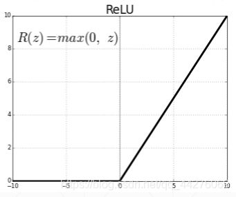
H = r e l u ( X W + b ) H=relu(XW+b) H=relu(XW+b)
一般最后一层的激活函数不是ReLU,也可以不加激活函数
用梯度下降法找到一组(W,b)使得对于一个新的X,其pred 接近Y
共有三组参数: [ W 1 , W 2 , W 3 ] [W_1,W_2,W_3] [W1,W2,W3] [ b 1 , b 2 , b 3 ] [b_1,b_2,b_3] [b1,b2,b3]
取概率最大的元素所对应的标签:argmax(pred)
识别步骤
加载数据
# -------------------------------------------- step 1/5 : 加载数据 -------------------------------------------
batch_size = 512
train_loader = torch.utils.data.DataLoader(
    torchvision.datasets.MNIST('mnist_data', train=True, download=True,   #download:如果当前文件没有数据,就要下载
            #加载mnist数据集,给出下载路径  train决定下载的是60k的训练数据,还是10k的测试数据
                                transform = torchvision.transforms.Compose([
                                     torchvision.transforms.ToTensor(),  #转换格式
                                     torchvision.transforms.Normalize(
                                         (0.1307,),(0.3081,))
                                    ])),
    batch_size = batch_size, shuffle = True)  #shuffle 随机打散

test_loader = torch.utils.data.DataLoader(
    torchvision.datasets.MNIST('mnist_data/', train=False, download=True,   #download:如果当前文件没有数据,就要下载
            #加载mnist数据集,给出下载路径  train决定下载的是60k的训练数据,还是10k的测试数据
                                transform = torchvision.transforms.Compose([
                                     torchvision.transforms.ToTensor(),  #转换格式
                                     torchvision.transforms.Normalize(
                                         (0.1307,),(0.3081,))
                                    ])),
    batch_size = batch_size, shuffle = False)  #shuffle 随机打散
从训练集中选一个样本:
x, y = next(iter(train_loader))
print(x.shape, y.shape)
输出为:
torch.Size([512, 1, 28, 28]) torch.Size([512])
结果为512张图片,单通道,28行28列,标签也为512个
Normalize归一化处理结果展示:
print(x.shape, y.shape, x.min(), x.max())
输出:
torch.Size([512, 1, 28, 28]) torch.Size([512]) tensor(-0.4242) tensor(2.8215)
最小值和最大值由[0, 1]变为[-0.4242, 2.8215]
构建网络模型
# ------------------------------------ step 2/5 : 定义网络 ------------------------------------
class Net(nn.Module):
    def __init__(self):
        super(Net, self).__init__()
        # xw+b
        self.fc1 = nn.Linear(28*28, 256)
        self.fc2 = nn.Linear(256,64)
        self.fc3 = nn.Linear(64,10)  #最后的输出要和类别数一样

    def forward(self, x):
        """计算过程"""
        #x:[batch, 1 , 28, 28]
        #H1=relu(xw1+b1)
        x = F.relu(self.fc1(x))    #经过第一层,加入激活函数
        # H2=relu(H1w2+b2)
        x = F.relu(self.fc2(x))
        # H3=H2w3+b3
        x = self.fc3(x)
        return x
训练
 # ------------------------------- step 3/5 : 定义损失函数和优化器进行训练 ------------------------------------
net = Net()
#定义优化器  #net.parameters()会返回[w1,b1,w2,b2,w3,b3]待优化的权值,
optimizer = optim.SGD(net.parameters(),lr=0.01, momentum=0.9)
train_loss = []
for epoch in range(3):    #迭代3次
    for batch_idx, (x,y) in enumerate(train_loader):  #对数据集迭代一次
      # x:[batch, 1 , 28, 28], y=[512]
      x = x.view(x.size(0), 28*28)
      # 把x打平 [batch, 1 , 28, 28]=》[b,784]
      out = net(x)
      #  =>[b,10]
      y_onehot = one_hot(y)
      #loss = 均方误差(out - y_onehot)^2 损失函数
      loss = F.mse_loss(out, y_onehot)

      optimizer.zero_grad()   #梯度清零
      loss.backward()     #计算梯度
      #w'= w -lr*grad
      optimizer.step()   #梯度更新 w,b 的更新

      train_loss.append(loss.item())   #转化为数值类型

      #每隔10个batch打印一下loss
      if batch_idx % 10 == 0:
          print(epoch, batch_idx, loss.item())

plot_curve(train_loss)
#得到了较优的[w1,b1,w2,b2,w3,b3]
输出:
2 110 0.031515102833509445

测试
# ------------------------------------ step 4/5 : 测试 ------------------------------------
total_corrent = 0
for x,y in test_loader:
    x = x.view(x.size(0), 28*28)
    out = net(x)
    #out :[b,10]  预测值:返回向量中较大的数的索引[0.1,0.8……]返回1
    pred = out.argmax(dim=1)
    #正确值
    corrent = pred.eq(y).sum().float().item()
#pred.eq(y)和真实的y进行比较,对的为1,把对的总个数累加转化为float类型,通过item转化为数值类型
    total_corrent += corrent
total_num = len(test_loader.dataset)
acc = total_corrent / total_num
print('test accuracy:',acc)

#取一个样本进行展示
x,y = next(iter(test_loader))
out = net(x.view(x.size(0), 28*28))
pred = out.argmax(dim=1)
plot_image(x, pred, 'test')
输出:
test accuracy: 0.8861

加载包
import torch
from torch import nn
from torch.nn import functional as F
from torch import optim
import torchvision
from matplotlib import pyplot as plt
from utils import plot_image,plot_curve, one_hot
utils.py
import torch
from matplotlib import pyplot as plt

def plot_curve(data):
    """绘制下降曲线(loss下降的过程)"""
    fig = plt.figure()
    plt.plot(range(len(data)), data, color = 'red')
    plt.legend(['value'],loc = 'upper right')
    plt.xlabel('step')
    plt.ylabel('value')
    plt.show()

def plot_image(img, label, name):
    """绘制图片"""
    fig = plt.figure()
    for i in range(6):
        plt.subplot(2, 3, i+1)
        plt.tight_layout()
        plt.imshow(img[i][0]*0.3081+0.1307, cmap='gray', interpolation='none')
        plt.title("{}: {}".format(name, label[i].item()))
        plt.xticks([])
        plt.yticks([])
    plt.show()

def one_hot(label, depth=10):
    """one_hot编码"""
    out = torch.zeros(label.size(0), depth)
    idx = torch.LongTensor(label).view(-1,1)
    out.scatter_(dim=1, index=idx, value=1)
    return out