There are various metrics that we can use to evaluate the performance of ML algorithms, classification as well as regression algorithms. We must carefully choose the metrics for evaluating ML performance because,
我们可以使用各种指标来评估ML算法,分类以及回归算法的性能。 我们必须谨慎选择评估ML性能的指标,因为,
- How the performance of ML algorithms is measured and compared will be dependent entirely on the metric we choose. ML算法的性能如何衡量和比较将完全取决于我们选择的指标。
- How we weight the importance of various characteristics in the result will be influenced completely by the metric we choose. 我们如何权衡各种特征在结果中的重要性,将完全取决于我们选择的指标。
The metrics that you choose to evaluate your machine learning model are very important. Choice of metrics influences how the performance of machine learning algorithms is measured and compared.
您选择用来评估机器学习模型的指标非常重要。 度量标准的选择会影响如何衡量和比较机器学习算法的性能。
内容 (Contents)
1.Performance Metrics for Classification Problems
1.分类问题的绩效指标
2.Performance Metrics for Regression Problems
2回归问题的绩效指标
3.Distribution of Errors
3,错误分布
分类问题的绩效指标 (Performance Metrics for Classification Problems)
1.准确性 (1. Accuracy)
Accuracy is the most intuitive performance measure and it is simply a ratio of correctly predicted observation to the total observations.
准确性是最直观的性能指标,它只是正确预测的观测值与总观测值的比率。
As a heuristic, or rule of thumb, accuracy can tell us immediately whether a model is being trained correctly and how it may perform generally. However, it does not give detailed information regarding its application to the problem.
作为一种启发法或经验法则,准确性可以立即告诉我们模型是否被正确训练以及其总体性能如何。 但是,它没有提供有关此问题的应用的详细信息。
If we have high accuracy then our model is best. Yes, accuracy is a great measure but only when we have symmetric datasets where values of positive and negative classes are almost the same.
如果我们具有高精度,那么我们的模型是最好的。 是的,准确性是一个很好的衡量标准,但是只有当我们拥有对称数据集时,正类别和负类别的值几乎相同。
When data is imbalanced, Accuracy is not the best measure and accuracy cannot use the probability score.
当数据不平衡时 ,准确性不是最佳度量,准确性也不能使用概率分数。
Ex: In our Amazon food review sentiment analysis example with 100 reviews, 10 people have said the review is positive. Let’s assume our model is very bad and predicts every review is positive. For this, it has classified those 90 people negative reviews as positive and 10 positive reviews as negative reviews. Now even though the model is terrible at predicting reviews, The accuracy of such a bad model is also 90%.
例:在我们的100条评论的亚马逊食品评论情绪分析示例中,有10个人说评论是肯定的。 让我们假设我们的模型非常糟糕,并预测每个评论都是正面的。 为此,它将90个人的负面评论归为正面,将10个人的负面评论归为负面。 现在,即使该模型在预测评论方面很糟糕,这种不良模型的准确性也高达90%。
2.混淆矩阵 (2. Confusion Matrix)
The Confusion matrix is one of the most intuitive and easiest metrics used for finding the correctness and accuracy of the model. It is used for the Classification problem where the output can be of two or more types of classes.
混淆矩阵是用于查找模型的正确性和准确性的最直观,最简单的指标之一。 它用于分类问题,其中输出可以是两种或多种类型的类。
Confusion Matrix cannot process the probability score.
混淆矩阵无法处理概率得分。
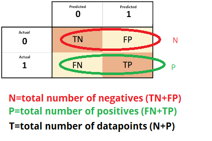
A confusion matrix is an N X N matrix, where N is the number of classes being predicted. For the problem in hand, if we have N=2, and hence we get a 2 X 2 matrix.
混淆矩阵是NXN矩阵,其中N是要预测的类别数。 对于手头的问题,如果我们有N = 2,则得到2 X 2矩阵。
Let’s assume in our Amazon Food reviews label to our target variable:1: When a person says the review is Positive.
让我们在我们的Amazon Food评论标签中假设目标变量为: 1 :当某人说评论为肯定。
0: When a person says the review is Negative.
0:当某人说评论为负面时。
The confusion matrix is a table with two dimensions (“Actual” and “Predicted”), and sets of “classes” in both dimensions. Our Actual classifications are rows and Predicted ones are Columns.
混淆矩阵是一个具有两个维度(“实际”和“预测”)的表,并且在两个维度中都有“类别”的集合。 我们的实际分类是行,预测的是列。
The Confusion matrix in itself is not a performance measure as such, but almost all of the performance metrics are based on the Confusion Matrix and the numbers inside it.
混淆矩阵本身并不是一个性能指标,但是几乎所有性能指标都是基于混淆矩阵及其内部数字的。
Explanation of the terms associated with confusion matrix are as follows,
与混淆矩阵相关的术语的解释如下,
True Negatives (TN) − It is the case when both the actual class and predicted class of data point is 0.
真负数(TN) -数据点的实际类别和预测类别均为0的情况。
Ex: The case where a review is actually negative(0) and the model classifying this review as negative(0) comes under True Negative.
例如:评论实际上是负面的(0),并且将该评论归为负面(0)的模型属于True Negative。
False Positives (FP) − It is the case when the actual class of data point is 0 and the predicted class of data point is 1.
误报(FP) -实际数据点类别为0而预测数据点类别为1。
Ex: The case where a review is actually negative(0) and the model classifying this review as positive(1) comes under False Positive.
例如:评论实际上是负面的(0),并且将该评论归为正面(1)的模型属于误报。
False Negatives (FN) − It is the case when the actual class of data point is 1 and the predicted class of data point is 0.
假阴性(FN) -数据点的实际类别为1而数据点的预测类别为0的情况。
Ex: The case where a review is actually positive(1) and the model classifying this review as negative(0) comes under False Negative.
例如:评论实际上是肯定的(1)并且将该评论归为否定(0)的模型属于假否定。
True Positives (TP) − It is the case when both the actual class and predicted class of data point is 1.
真实正值(TP) -数据点的实际类别和预测类别均为1。
Ex: The case where a review is actually positive(1) and the model classifying this review as positive(1) comes under True positive.
例:评论实际上是肯定的(1)且将该评论归为肯定(1)的模型属于“真正肯定”。
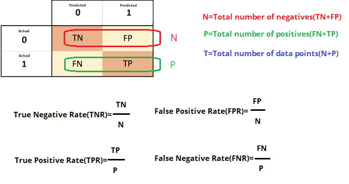
N is the total number of negatives in our given data and P is the total number of positives in our data shown in the below image.
N是给定数据中的负数总数,P是下图中所示的数据中的正数总数。
Accuracy in terms of the confusion matrix given by in classification problems is the number of correct predictions made by the model over all kinds of predictions made.
在分类问题中给出的混淆矩阵方面的准确性是模型在做出的所有预测中做出的正确预测的数量。
We can use the accuracy_score function of sklearn.metrics to compute the accuracy of our classification model.
我们可以用sklearn.metrics的accuracy_score函数来计算我们的分类模型的准确性。
For a good model, the True Positive Rate and True Negative Should be high, and the False Positive Rate and False Negative Rate Should be low.
对于一个好的模型,真正率和真负率应该高,假正率和假负率应该低。
Some examples
一些例子
False Positive (FP) moves a trusted email to junk in an anti-spam engine.False Negative (FN) in medical screening can incorrectly show disease absence when it is actually positive.
误报(FP)将受信任的电子邮件发送到反垃圾邮件引擎中的垃圾邮件。医学筛查中的误报(FN)可能在实际为阳性时错误地表明没有疾病。
精度,召回(或)灵敏度,特异性,F1-Score (Precision ,Recall (or) sensitivity ,Specificity,F1-Score)
Precision and Recall are extensively used in information retrieval problems when we have a large corpus of text data.
当我们拥有大量文本数据集时,Precision和Recall广泛用于信息检索问题。
Precision: Precision tells about us of all the points model predicted to be positive, what percentage of points are actually positive.
精度:精度告诉我们所有预测为正的点模型,实际上是多少点是正的。
Precision is about being precise. So even if we managed to capture only one cancer case, and we captured it correctly, then we are 100% precise.
精确就是精确。 因此,即使我们仅成功捕获了一个癌症病例,并且我们正确地捕获了该癌症病例,我们也可以做到100%精确。
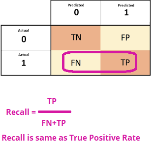
Recall (or) Sensitivity (or) True Positive Rate: Recall tells about us of all the points are actually belong to the positive points, how many points are to be predicted as positive points.
召回(或)敏感度(或)真实正比率:召回告诉我们所有点实际上都属于正点,要预测多少点为正点。
Recall is not so much about capturing cases correctly but more about capturing all cases that have “cancer” with the answer as “cancer”. So if we simply always say every case as “cancer”, we have 100% recall.
召回并不是正确地捕获案例,而是捕获所有具有“癌症”且答案为“癌症”的案例。 因此,如果我们只是总是将每种情况都说成是“癌症”,那么我们有100%的回忆率。
So basically if we want to focus more on minimizing False Negatives, we would want our Recall to be as close to 100% as possible without precision being too bad and if we want to focus on minimizing False positives, then our focus should be to make Precision as close to 100% as possible.
因此,基本上,如果我们想将更多的精力集中在最小化误报上,那么我们希望召回率尽可能地接近100%,而精度又不会太差;并且如果我们想将精力集中在最小化误报上,那么我们的重点应该放在精度尽可能接近100%。
It is clear that recall gives us information about a classifier’s performance with respect to false negatives (how many did we miss), while precision gives us information about its performance with respect to false positives(how many did we caught).
很明显,召回为我们提供了有关分类器在误报方面的表现的信息(我们错过了多少),而精确度 向我们提供有关误报方面性能的信息(我们捕获了多少)。
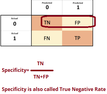
Specificity (or) True Negative Rate: Specificity, in contrast, to recall, may be defined as the number of negatives returned by our ML model. We can easily calculate it by confusion matrix with the help of following formula
特异性(或)真实阴性率:相比之下,回忆性可以将特异性定义为我们的ML模型返回的阴性数。 我们可以借助以下公式轻松地通过混淆矩阵进行计算
F1-Score: We don’t really want to carry both Precision and Recall in our pockets every time we make a model for solving a classification problem. So it’s best if we can get a single score that kind of represents both Precision(P) and Recall(R).
F1-Score:每次创建模型来解决分类问题时,我们都不希望同时携带Precision和Recall。 因此,最好是获得一个表示Precision(P)和Recall(R)的单一分数。
This score will give us the harmonic mean of precision and recall. Mathematically, the F1-Score is the weighted average of precision and recall. The best value of F1-Score would be 1 and the worst would be 0. F1-Score is having an equal relative contribution of precision and recall.
该分数将为我们提供精确度和查全率的调和平均值。 从数学上讲,F1-分数是精度和召回率的加权平均值。 F1-Score的最佳值将是1,最差的将是0。F1-Score在精度和召回率上的相对贡献相等。
For Multi-Class Classification, we use similar metrics like F1-Score there are
对于多类别分类,我们使用类似F1-Score的指标
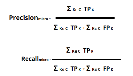
Micro F1-Score: Micro F1-score (short for micro-averaged F1 score) is used to assess the quality of multi-label binary problems. It measures the F1-score of the aggregated contributions of all classes.
Micro F1分数: Micro F1分数(Micro-F1平均分数的缩写)用于评估多标签二进制问题的质量。 它衡量所有类别的总贡献的F1得分。
If you are looking to select a model based on a balance between precision and recall, don’t miss out on assessing your F1-scores.
如果您希望基于精度和召回率之间的平衡来选择模型,请不要错过评估F1得分的机会。
Micro F1-score 1 is the best value (perfect micro-precision and micro-recall), and the worst value is 0. Note that precision and recall have the same relative contribution to the F1-score.
Micro F1分数1是最佳值(完美的微精度和微召回率 ),最差值为0。请注意,精度和召回率对F1分数具有相同的相对贡献。
C is the Number of Classes and K ∈ C.
C是类数, K∈C。
Micro F1-score is defined as the harmonic mean of the precision and recall:
Micro F1分数定义为精度和查全率的谐波平均值:
Micro-averaging F1-score is performed by first calculating the sum of all true positives, false positives, and false negatives over all the labels. Then we compute the micro-precision and micro-recall from the sums. And finally, we compute the harmonic mean to get the micro F1-score.
通过首先计算所有标签上所有真阳性,假阳性和假阴性的总和来执行F1分数的微平均。 然后,我们根据这些和计算出微精度和微召回率。 最后,我们计算谐波平均值以获得微F1分数。
Micro-averaging will put more emphasis on the common labels in the data set since it gives each sample the same importance. This may be the preferred behavior for multi-label classification problems.
微观平均将更加重视数据集中的通用标签,因为它赋予每个样本相同的重要性。 对于多标签分类问题,这可能是首选的行为。
Macro F1-Score: Macro F1-score (short for macro-averaged F1 score) is used to assess the quality of problems with multiple binary labels or multiple classes.
宏F1分数:宏F1分数(宏F1分数的缩写)用于评估具有多个二进制标签或多个类别的问题的质量。
Macro F1-score is defined as the average harmonic mean of precision and recall of each class:
宏F1分数定义为每个类别的精度和召回率的平均谐波平均值:
C is the Number of Classes and K ∈ C.
C是类数, K∈C。
Macro F1-score will give the same importance to each label/class. It will be low for models that only perform well on the common classes while performing poorly on the rare classes.
宏F1分数将对每个标签/类给予相同的重视。 对于仅在普通类上表现良好而在稀有类上表现较差的模型,该值将较低。
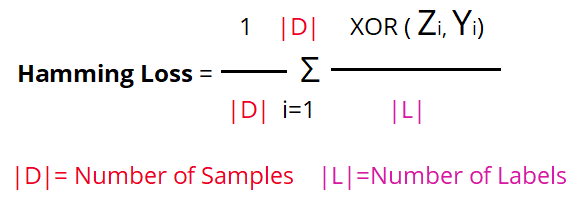
Hamming Loss: Hamming loss is the fraction of wrong labels to the total number of labels. In multi-class classification, the hamming loss is calculated as the hamming distance between actual and predictions.
汉明丢失:汉明丢失是错误标签占标签总数的比例。 在多类分类中,汉明损失被计算为实际和预测之间的汉明距离。
This is a loss function, so the optimal value is zero.
这是一个损失函数,因此最佳值为零。
3.接收机工作特性曲线 (3. Receiver Operating Characteristics Curve)
Receiver-operating characteristic (ROC) analysis was originally developed during World War II to analyze classification accuracy in differentiating signals from noise in radar detection. Recently, the methodology has been adapted to several clinical areas heavily dependent on screening and diagnostic tests, in particular, laboratory testing, epidemiology, radiology, and bioinformatics.
接收机工作特性(ROC)分析最初是在第二次世界大战期间开发的,用于分析区分雷达检测中的信号与噪声的分类精度。 最近,该方法已经适应于严重依赖筛查和诊断测试的多个临床领域,特别是实验室测试,流行病学,放射学和生物信息学。
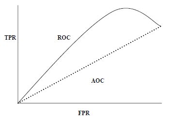
A Receiver Operating Characteristic (ROC) Curve is a way to compare diagnostic tests. It is a plot of the True Positive Rate against the False Positive Rate.
接收器工作特性(ROC)曲线是比较诊断测试的一种方法。 它是真实肯定率与错误肯定率的曲线图。
AUC (Area Under Curve)-ROC (Receiver Operating Characteristic) is a performance metric, based on varying threshold values, for classification problems. As the name suggests, ROC is a probability curve, and AUC measures the separability.
AUC(曲线下面积)-ROC(接收器工作特性)是一种性能指标,基于变化的阈值,用于分类问题。 顾名思义,ROC是一条概率曲线,而AUC则测量可分离性。
ROC is used in binary Classification. To compute ROC first we want to do
ROC用于二进制分类。 首先要计算ROC
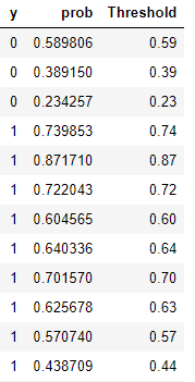
- Getting classification model probability predictions. The probabilities usually range between 0 and 1. 获取分类模型概率预测。 概率通常在0到1之间。
- AUC cannot care about the probability score it only cares about the sorted order of data. AUC不在乎概率分数,它只在乎数据的排序顺序。
- Sort the data into discrete order. 将数据按离散顺序排序。
- The next step is to find a threshold to classify the probabilities. 下一步是找到一个阈值以对概率进行分类。
- To plot the ROC curve, we need to calculate the TPR and FPR for different thresholds using a confusion matrix. 要绘制ROC曲线,我们需要使用混淆矩阵来计算不同阈值的TPR和FPR。
- For each threshold, we plot the FPR value in the x-axis and the TPR value in the y-axis. We then join the dots with a line. 对于每个阈值,我们在x轴上绘制FPR值,在y轴上绘制TPR值。 然后,我们用一条线将点连接起来。
In simple words, the AUC-ROC metric will tell us about the capability of the model in distinguishing the classes. Higher the AUC, the better the model.
简而言之,AUC-ROC度量标准将告诉我们该模型区分类的能力。 AUC越高,模型越好。
The ROC curve is plotted with TPR against the FPR where TPR is on the y-axis and FPR is on the x-axis.
用TPR相对FPR绘制ROC曲线,其中TPR在y轴上,FPR在x轴上。
An excellent model has AUC near to the 1 which means it has a good measure of separability. A poor model has AUC near to the 0 which means it has the worst measure of separability. In fact, it means it is reciprocating the result. It is predicting 0s as 1s and 1s as 0s. And when AUC is 0.5, it means the model has no class separation capacity whatsoever.
出色的模型的AUC接近1,这意味着它具有很好的可分离性度量。 较差的模型的AUC接近于0,这意味着它具有最差的可分离性度量。 实际上,这意味着它在回报结果。 它预测0s为1s,1s为0s。 当AUC为0.5时,表示该模型没有任何类别分离能力。
4.对数概率(对数损失) (4. Log probability (Log Loss))
Log Loss is the most important classification metric based on probabilities.
对数丢失是基于概率的最重要的分类指标。
If the model gives us the probability score, Log-loss is the best performance measure for both binary and Multi classification.
如果模型为我们提供了概率得分,则对数损失是二进制分类和多分类分类的最佳性能度量。
The goal of our machine learning models is to minimize this value. A perfect model would have a log loss of 0.
我们的机器学习模型的目标是最小化此值。 理想模型的对数损失为0。
It’s hard to interpret raw log-loss values, but log-loss is still a good metric for comparing models. For any given problem, a lower log-loss value means better predictions.
很难解释原始的对数损失值,但是对数损失仍然是比较模型的良好指标。 对于任何给定的问题,较低的对数损失值意味着更好的预测。
Log loss quantifies the average difference between predicted and expected probability distributions.
对数损失量化了预测概率分布与预期概率分布之间的平均差异。
回归问题的绩效指标 (Performance Metrics for Regression Problems)
1.R²或确定系数 (1. R² or Coefficient of Determination)
It is known as the coefficient of determination. It is a statistical measure of how close the data are to the fitted regression line Or indicates the goodness of fit of a set of predictions to the actual values. The value of R² lies between 0 and 1 where 0 means no-fit and 1 means perfectly-fit.
这就是确定系数。 它是一种统计度量,用于衡量数据与拟合的回归线的接近程度,或者指示一组预测与实际值的拟合度。 R²的值介于0和1之间,其中0表示不适合,而1表示完全适合。
R-squared is calculated by dividing the sum of squares of residuals (SSres) from the regression model by the total sum of squares (SStot) of errors from the average model and then subtract it from 1.
R平方是通过从平均模型除以从回归模型的残差(SSres)平方和由平方误差的总和(SStot)来计算,然后从1中减去它。
Where SSE is the Sum of Square of Residuals. Here residual is the difference between the predicted value and the actual value.it is also called an error.
其中SSE是残差平方和。 此处残差是预测值与实际值之间的差,也称为误差。
And SST is the Total Sum of Squared error using a simple mean model.
SST是使用简单均值模型的平方误差总和。
An R-squared value of 0.81, tells that the input variables explain 81 % of the variation in the output variable. The higher the R squared, the more variation is explained by the input variables and better is the model.
R平方值为0.81,表明输入变量解释了输出变量变化的81%。 R平方越高,输入变量说明的变化越大,并且模型越好。
2. 调整后的R² (2. Adjusted R²)
The limitation of R-squared is that it will either stay the same or increases with the addition of more variables, even if they do not have any relationship with the output variables.
R平方的局限性在于 ,即使它们与输出变量没有任何关系,R平方也会随着添加更多变量而保持不变或增加。
To overcome this limitation, Adjusted R-square comes into the picture as it penalizes you for adding the variables which do not improve your existing model.
为了克服此限制,调整后的R平方会出现在图片中,因为它会因添加无法改善现有模型的变量而受到惩罚。
Adjusted R² depicts the same meaning as R² but is an improvement of it. R² suffers from the problem that the scores improve on increasing terms even though the model is not improving which may misguide the researcher. Adjusted R² is always lower than R² as it adjusts for the increasing predictors and only shows improvement if there is a real improvement.
调整后的R²表示与R²相同的含义,但它是对R²的改进。 R 2的问题在于,即使模型没有改进,分数也会随着增加而提高,这可能会误导研究人员。 调整后的R²始终低于R²,因为它会针对不断增长的预测指标进行调整,并且只有在真正改善的情况下才会显示出改善。
Hence, if you are building Linear regression on multiple variables, it is always suggested that you use Adjusted R-squared to judge the goodness of the model.
因此,如果要在多个变量上建立线性回归,则始终建议您使用调整后的R平方来判断模型的优劣。
3.均方误差(MSE) (3. MEAN SQUARE ERROR (MSE))
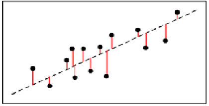
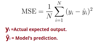
MSE or Mean Squared Error is one of the most preferred metrics for regression tasks. It is simply the average of the squared difference between the target value and the value predicted by the regression model.
MSE或均方误差是回归任务最优选的指标之一。 它只是目标值与回归模型预测的值之间的平方差的平均值。
As it squares the differences, it penalizes even a small error which leads to over-estimation of how bad the model is. It is preferred more than other metrics because it is differentiable and hence can be optimized better.
当平方差异时,它甚至会惩罚一个很小的误差,从而导致对模型的严重程度的高估。 与其他度量相比,它更可取,因为它是可区分的,因此可以更好地进行优化。
Here, the error term is squared and thus more sensitive to outliers.
在这里,误差项是平方的,因此对异常值更为敏感。
3.根均方误差(RMSE) (3. ROOT MEAN SQUARE ERROR (RMSE))
RMSE is the most widely used metric for regression tasks and is the square root of the averaged squared difference between the target value and the value predicted by the model.
RMSE是用于回归任务的最广泛使用的度量标准,是目标值与模型预测的值之间的平均平方差的平方根。
MSE includes squared error terms, we take the square root of the MSE, which gives rise to Root Mean Squared Error (RMSE).
MSE包含平方误差项,我们取MSE的平方根,这将引起均方根误差(RMSE)。
RMSE is highly affected by outlier values. Hence, make sure you’ve removed outliers from your data set prior to using this metric.
RMSE受异常值的影响很大。 因此,在使用此指标之前,请确保已从数据集中删除了异常值。
4.平均绝对误差(MAE) (4. Mean Absolute Error (MAE))
It is the simplest error metric used in regression problems. It is basically the sum of the average of the absolute difference between the predicted and actual values.
它是用于回归问题的最简单的误差度量。 它基本上是预测值与实际值之间的绝对差的平均值之和。
In simple words, with MAE, we can get an idea of how wrong the predictions were
简而言之,借助MAE,我们可以了解预测的错误程度
5.中值绝对偏差(MADE) (5. Median Absolute Deviation Error(MADE))
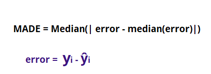
Median Absolute Deviation: The median absolute deviation(MAD) is a robust measure of how to spread out a set of data is. The variance and standard deviation are also measures of spread, but they are more affected by extremely high or extremely low values and non-normality.
中位数绝对偏差 :中位数绝对偏差(MAD)是衡量如何分散一组数据的可靠方法。 方差和标准偏差也是点差的度量,但是它们受极高或极低值以及非正态性的影响更大。
First, find the median of error, then subtract this median from each error, then take the absolute value of these differences, Find the median of these absolute differences.
首先,找到误差的中位数,然后从每个误差中减去该中位数,然后取这些差异的绝对值,然后找到这些绝对差异的中位数。
错误分布 (Distribution of Errors)
To understand errors, for every point compute error and distribute in PDF and CDF.
要了解错误,请为每个点计算错误并以PDF和CDF进行分发。
The probability distribution for a random error that is as likely to move the value in either direction is called a Gaussian distribution.
可能在任一方向上移动该值的随机误差的概率分布称为高斯分布 。
In the above image, most of the errors are small, very few errors are large, smaller errors better for regression.
在上图中,大多数误差很小,很少的误差很大,较小的误差更适合回归。
In the above image, 99 % of errors are < 0.1 and 1 % of errors are ≥ 0.1.
在上图中,99%的误差<0.1,1%的误差≥0.1。
If we compare the errors of the two models, the red color model is M1 is having 95 % of errors below 0.1 and the blue color model is M2 is having 80% of errors are below 0.1. From this, we conclude the M1 is better than M2.
如果我们比较两个模型的误差,则红色模型为M1,其95%的误差低于0.1,蓝色模型为M2,其80%的误差低于0.1。 据此,我们得出结论,M1优于M2。
I Performed some tasks for Classification and Regression from the scratch show in the below image.
从下图开始,我从头开始执行一些分类和回归任务。
For complete code to understand visit my GitHub link.
要了解完整的代码,请访问我的GitHub链接。
结论 (Conclusion)
In this post, we discovered about the various metrics used in Classification and Regression analysis in Machine Learning.
在这篇文章中,我们发现了有关机器学习的分类和回归分析中使用的各种度量。
翻译自: https://medium.com/analytics-vidhya/performance-metrics-for-machine-learning-models-80d7666b432e


