pytorch实现AlexNet,在mnist数据集上实验,用精确率、召回率等指标评估,并绘制PR、ROC曲线
一、导入需要的模块
import torch
import prettytable
import numpy as np
import matplotlib.pyplot as plt
from torch import nn
from torch.utils.data import Dataset
from torch.utils import data
from torchvision import datasets
from torchvision.transforms import ToTensor
from torchvision import transforms
from torch.utils.data import DataLoader
from torch.nn import functional as F
from torchsummary import summary
from torch.utils.tensorboard import SummaryWriter
二、准备数据集
#获取数据集
trans = [transforms.ToTensor()]
trans.insert(0, transforms.Resize(224))
trans = transforms.Compose(trans)
batch_size = 256

training_data = datasets.MNIST(
    root="./data",
    train=True,
    download=True,
    transform=trans
)

test_data = datasets.MNIST(
    root="./data",
    train=False,
    download=True,
    transform=trans
)

train_iter = data.DataLoader(training_data, batch_size, shuffle=True,
                        num_workers=2)
test_iter = data.DataLoader(test_data, batch_size, shuffle=False,
                        num_workers=2)

train_features, train_labels = next(iter(train_iter))
print(f"Feature batch shape: {train_features.size()}")
print(f"Labels batch shape: {train_labels.size()}")
print(f"batch size:{len(iter(train_iter))}")
输出:
Feature batch shape: torch.Size([256, 1, 224, 224])
Labels batch shape: torch.Size([256])
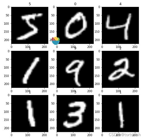
batch size:235三、数据集可视化
#随机展示训练集中的九张图片
figure = plt.figure(figsize=(8, 8))
sample_idx = torch.randint(len(training_data), size=(9,))
row, column = 0, 0
for i, pict_index in enumerate(sample_idx):
    img, label = training_data[i]
    figure.add_subplot(3, 3, i+1)
    plt.title(str(label))
    plt.imshow(img.squeeze(), cmap="gray")
plt.show()
输出:
四、定义AlexNet
这里严格按照Alex Krizhevsky的论文《ImageNet Classification with Deep Convolutional Neural Networks》定义AlexNet。
当然如果想要省事,也可以直接从torchvision中导入~~~
class AlexNet(nn.Module):
    def __init__(self):
        super(AlexNet, self).__init__()
        self.conv1 = nn.Conv2d(1, 96, kernel_size=(11, 11), stride=4, padding=2)
        self.maxpool1 = nn.MaxPool2d(kernel_size=(3, 3), stride=2)
        self.conv2 = nn.Conv2d(96, 256, kernel_size=(5, 5), stride=1, padding=2)
        self.maxpool2 = nn.MaxPool2d(kernel_size=(3, 3), stride=2)
        self.conv3 = nn.Conv2d(256, 384, kernel_size=(3, 3), padding=1)
        self.conv4 = nn.Conv2d(384, 384, kernel_size=(3, 3), padding=1)
        self.conv5 = nn.Conv2d(384, 256, kernel_size=(3, 3), padding=1)
        self.maxpool3 = nn.MaxPool2d(kernel_size=(3, 3), stride=2)
        self.flatten = nn.Flatten()
        self.linear1 = nn.Linear(9216, 4096)
        self.dropout1 = nn.Dropout(0.5)
        self.linear2 = nn.Linear(4096, 4096)
        self.dropout2 = nn.Dropout(0.5)
        self.linear3 = nn.Linear(4096, 10)

    def forward(self, x):
        out_conv1 = F.relu(self.conv1(x))
        out_pool1 = self.maxpool1(out_conv1)
        out_conv2 = F.relu(self.conv2(out_pool1))
        out_pool2 = self.maxpool2(out_conv2)
        out_conv3 = F.relu(self.conv3(out_pool2))
        out_conv4 = F.relu(self.conv4(out_conv3))
        out_conv5 = F.relu(self.conv5(out_conv4))
        out_pool3 = self.maxpool3(out_conv5)

        flatten_x = self.flatten(out_pool3)
        out_linear1 = F.relu(self.linear1(flatten_x))
        out_dropout1 = self.dropout1(out_linear1)
        out_linear2 = F.relu(self.linear2(out_dropout1))
        out_dropout2 = F.relu(out_linear2)
        out_linear3 = F.relu(self.linear3(out_dropout2))
        return out_linear3
五、定义训练循环、测试循环、初始化超参数
#定义超参数,采用SGD作为优化器
learning_rate = 0.001
batch_size = 256
optimizer = torch.optim.SGD(model.parameters(), lr=learning_rate)
device = 'cuda' if torch.cuda.is_available() else 'cpu'
loss_fn = nn.CrossEntropyLoss()
model.to(device)
loss_list = []
acc_list = []
epoch_num = []

def init_weights(m):
        if type(m) == nn.Linear or type(m) == nn.Conv2d:
            nn.init.xavier_uniform_(m.weight)

#定义训练循环和测试循环
def train_loop(dataloader, model, loss_fn, optimizer, epoch):
    size = len(dataloader.dataset)
    for t in range(epoch):
        print(f"Epoch {t+1}\n-------------------------------")
        running_loss = 0
        for batch, (X, y) in enumerate(dataloader):
            X, y = X.to(device), y.to(device)
            pred = model(X)
            loss = loss_fn(pred, y)
            running_loss += loss
            # Backpropagation
            optimizer.zero_grad()
            loss.backward()
            optimizer.step()

            if batch % 50 == 49:
                writer.add_scalar('training loss',
                                running_loss / 50,
                                epoch * len(dataloader)+batch+1)

                loss, current = loss.item(), (batch+1) * len(X)
                loss_list.append(loss), epoch_num.append(t+current/size)
                print(f"loss: {loss:>7f}  [{current:>5d}/{size:>5d}]")
                running_loss = 0

        test_loop(test_iter, model, loss_fn)

def test_loop(dataloader, model, loss_fn):
    size = len(dataloader.dataset)
    num_batches = len(dataloader)
    test_loss, correct = 0, 0

    with torch.no_grad():
        for X, y in dataloader:
            X, y = X.to(device), y.to(device)
            pred = model(X)
            test_loss += loss_fn(pred, y).item()
            correct += (pred.argmax(1) == y).type(torch.float).sum().item()

    test_loss /= num_batches
    correct /= size
    acc_list.append(correct)
    print(f"Test Error: \n Accuracy: {(100*correct):>0.1f}%, Avg loss: {test_loss:>8f}")
六、建模完成,开始训练!
model.apply(init_weights)
writer = SummaryWriter()
train_loop(train_iter, model, loss_fn, optimizer, 30)
输出:
Epoch 1
-------------------------------
loss: 2.303341 [12800/60000]
loss: 2.303362 [25600/60000]
loss: 2.300716 [38400/60000]
loss: 2.300808 [51200/60000]
Test Error:
Accuracy: 11.5%, Avg loss: 2.300705
.........
.........
.........
Epoch 30
-------------------------------
loss: 0.075750 [12800/60000]
loss: 0.073634 [25600/60000]
loss: 0.110787 [38400/60000]
loss: 0.061658 [51200/60000]
Test Error:
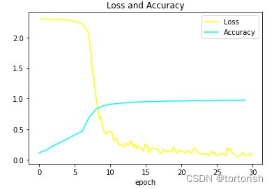
Accuracy: 97.4%, Avg loss: 0.081114七、模型评估及可视化
1、loss、accuracy曲线
#保存模型
torch.save(model.state_dict(), 'MnistOnAlexNet_epoch30.pkl')
#绘制损失和准确度曲线
plt.title('Loss and Accuracy')
plt.xlabel('epoch')
plt.plot(epoch_num, loss_list, 'yellow')
plt.plot(range(30), acc_list, 'cyan')
plt.legend(['Loss', 'Accuracy'])
plt.show()
结果:
2、输出精确率、召回率
#在测试集上评估模型
model.eval()
model.to('cpu')
pred_list = torch.tensor([])
with torch.no_grad():
    for X, y in test_iter:
        pred = model(X)
        pred_list = torch.cat([pred_list, pred])

test_iter1 = data.DataLoader(test_data, batch_size=10000, shuffle=False,
                        num_workers=2)
features, labels = next(iter(test_iter1))
print(labels.shape)
#输出每个类别的精确率和召回率
train_result = np.zeros((10, 10), dtype=int)
for i in range(len(test_data)):
train_result[labels[i]][np.argmax(pred_list[i])] += 1
result_table = prettytable.PrettyTable()
result_table.field_names = ['Type', 'Accuracy(精确率)', 'Recall(召回率)', 'F1_Score']
class_names = ['Zero', 'One', 'Two', 'Three', 'Four', 'Five', 'Six', 'Seven', 'Eight', 'Nine']
for i in range(10):
accuracy = train_result[i][i] / train_result.sum(axis=0)[i]
recall = train_result[i][i] / train_result.sum(axis=1)[i]
result_table.add_row([class_names[i], np.round(accuracy, 3), np.round(recall, 3),
np.round(accuracy * recall * 2 / (accuracy + recall), 3)])
print(result_table)结果:
+-------+------------------+----------------+----------+
|  Type | Accuracy(精确率) | Recall(召回率) | F1_Score |
+-------+------------------+----------------+----------+
|  Zero |      0.972       |     0.993      |  0.982   |
|  One  |      0.991       |     0.985      |  0.988   |
|  Two  |      0.983       |     0.976      |   0.98   |
| Three |      0.966       |     0.984      |  0.975   |
|  Four |      0.994       |     0.966      |   0.98   |
|  Five |      0.994       |      0.97      |  0.982   |
|  Six  |      0.988       |     0.981      |  0.985   |
| Seven |      0.982       |     0.965      |  0.974   |
| Eight |      0.954       |     0.983      |  0.968   |
|  Nine |      0.953       |     0.972      |  0.963   |
+-------+------------------+----------------+----------+
3、对十个类别分别绘制PR曲线和ROC曲线
#采用scikit-learn模块对10个类分别绘制PR曲线和ROC曲线
from sklearn.metrics import precision_recall_curve, roc_curve

for i in range(10):
    temp_true = []
    temp_probilities = []
    temp = 0

    for j in range(len(labels)):
        if i == labels[j]:
            temp = 1
        else:
            temp = 0
        temp_true.append(temp)
        temp_probilities.append(pred_probilities[j][i])

    precision, recall, threshholds = precision_recall_curve(temp_true, temp_probilities)
    fpr, tpr, thresholds = roc_curve(temp_true, temp_probilities)

    plt.figure(figsize=(12, 6))
    plt.subplot(1, 2, 1)
    plt.xlabel('Precision')
    plt.ylabel('Recall')
    plt.title(f'Precision & Recall Curve (class:{i}) ')
    plt.plot(precision, recall, 'yellow')

    plt.subplot(1, 2, 2)
    plt.xlabel('Fpr')
    plt.ylabel('Tpr')
    plt.title(f'Roc Curve (class:{i})')
    plt.plot(fpr, tpr, 'cyan')
    plt.show()
结果:
第1类(数字1)的PR、ROC曲线
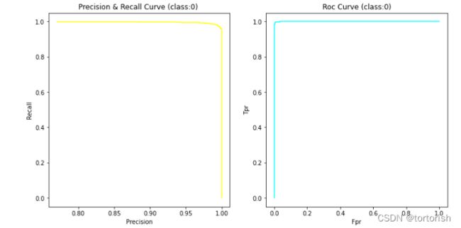
可以看到非常完美!
其他九个类别(2-9)也是一样的,每个类别都对应一张PR曲线图和ROC曲线图,这里因为篇幅原因就不放了。
代码完整版可以看github,数据集和预训练权重可以查看release分支:
https://github.com/tortorish/Pytorch_AlexNet_Mnist