深度学习之Alexnet学习笔记

声明：本文主要是谈谈对CNN中的Alexnet网络学习的感想，本人初学者，如有错误的地方欢迎指正。文章部分内容来源于网络诸位大神，所以如有相同的地方，望谅解。本文只适用于交流学习。文章后面是我利用Alexnet网络对MNIST数字识别进行训练的模型，并写了一个输入图片进行预测的程序。

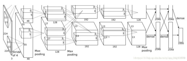
Alexnet网络训练了一个大规模的深度卷积神经网络来将ImageNet LSVRC-2010比赛中的包含120万幅高分辨率的图像数据集分为1000种不同类别。该神经网络包含6千万个参数和65万个神经元，包含了5个卷积层，其中有几层后面跟着最大池化（max-pooling）层，以及3个全连接层，最后还有一个1000路的softmax层。为了加快训练速度，该网络使用了不饱和神经元以及一种高效的基于GPU的卷积运算方法。为了减少全连接层的过拟合，该网络采用了最新的正则化方法“dropout”。

网络模型如图所示：

基于原文的解读,该网络主要优点有一下四点：

1、数据增强，提出"dropout"方法 （减少过拟合）

2、重叠pool池化（提高精度、不容易产生过拟合）

3、局部响应归一化（提高精度）

4、ReLU、两个GPU同时训练（提高速度）

下面我用训练MNIST数字识别的类型来谈谈对Alexnet网络的理解：

MNIST是一个简单的视觉计算数据集，它是像下面这样手写的数字图片：

每张图片还额外有一个标签记录了图片上数字是几，例如上面几张图的标签就是：5、0、4、1。 

本次将会展现如何训练一个模型来识别这些图片，最终实现模型对图片上的数字进行预测。

首先是对网络的结构分析，mnist数据是28*28的图片，扩展之后是（1,784）的数据，Alexnet网络第一层卷积神经网络是卷积层+池化层+norm，卷积网络是利用96个11*11*1的滤波器，卷积是都采用padding补齐，卷积后图片大小不变，池化层是2*2*1,步长为2，池化后图片大小缩小一半，代码如下：

# 定义卷积操作
def conv2d(name,x, W, b, strides=1):
    # Conv2D wrapper, with bias and relu activation
    x = tf.nn.conv2d(x, W, strides=[1, strides, strides, 1], padding='SAME')
    x = tf.nn.bias_add(x, b)
    return tf.nn.relu(x,name=name)  # 使用relu激活函数

# 定义池化层操作
def maxpool2d(name,x, k=2):
    # MaxPool2D wrapper
    return tf.nn.max_pool(x, ksize=[1, k, k, 1], strides=[1, k, k, 1],
                          padding='SAME',name=name)

# 规范化操作
def norm(name, l_input, lsize=4):
    return tf.nn.lrn(l_input, lsize, bias=1.0, alpha=0.001 / 9.0,
                     beta=0.75, name=name)

def alex_net(x, weights, biases, dropout):
    # 向量转为矩阵 Reshape input picture
    x = tf.reshape(x, shape=[-1, 28, 28, 1])

    # 第一层卷积
    # 卷积
    conv1 = conv2d('conv1', x, weights['wc1'], biases['bc1'])
    # 下采样
    pool1 = maxpool2d('pool1', conv1, k=2)
    # 规范化
    norm1 = norm('norm1', pool1, lsize=4)

Alexnet网络第二层：

# 第二层卷积
    # 卷积
    conv2 = conv2d('conv2', norm1, weights['wc2'], biases['bc2'])
    # 最大池化（向下采样）
    pool2 = maxpool2d('pool2', conv2, k=2)
    # 规范化
    norm2 = norm('norm2', pool2, lsize=4)

Alexnet网络第三层：

# 卷积
    conv3 = conv2d('conv3', norm2, weights['wc3'], biases['bc3'])
    # 规范化
    norm3 = norm('norm3', conv3, lsize=4)

Alexnet网络第四层：

  # 第四层卷积
    conv4 = conv2d('conv4', norm3, weights['wc4'], biases['bc4'])

 # 第五层卷积
    conv5 = conv2d('conv5', conv4, weights['wc5'], biases['bc5'])
    # 最大池化（向下采样）
    pool5 = maxpool2d('pool5', conv5, k=2)
    # 规范化
    norm5 = norm('norm5', pool5, lsize=4)

# 全连接层1
    fc1 = tf.reshape(norm5, [-1, weights['wd1'].get_shape().as_list()[0]])
    fc1 =tf.add(tf.matmul(fc1, weights['wd1']),biases['bd1'])
    fc1 = tf.nn.relu(fc1)
    # dropout
    fc1=tf.nn.dropout(fc1,dropout)

    # 全连接层2
    fc2 = tf.reshape(fc1, [-1, weights['wd2'].get_shape().as_list()[0]])
    fc2 =tf.add(tf.matmul(fc2, weights['wd2']),biases['bd2'])
    fc2 = tf.nn.relu(fc2)
    # dropout
    fc2=tf.nn.dropout(fc2,dropout)

    # 输出层
    out = tf.add(tf.matmul(fc2, weights['out']) ,biases['out'])
    return out

# 构建模型
pred = alex_net(x, weights, biases, keep_prob)

# 定义损失函数和优化器
cost = tf.reduce_mean(tf.nn.softmax_cross_entropy_with_logits(labels=y,logits=pred))
optimizer = tf.train.AdamOptimizer(learning_rate=learning_rate).minimize(cost)

# 评估函数
correct_pred = tf.equal(tf.argmax(pred,1), tf.argmax(y,1))
accuracy = tf.reduce_mean(tf.cast(correct_pred, tf.float32))

# 初始化变量
init = tf.global_variables_initializer()
saver=tf.train.Saver()
# 开启一个训练
with tf.Session() as sess:
    sess.run(init)
    step = 1
    # 开始训练，直到达到training_iters，即200000
    while step * batch_size < training_iters:
        #获取批量数据
        batch_x, batch_y = mnist.train.next_batch(batch_size)
        sess.run(optimizer, feed_dict={x: batch_x, y: batch_y, keep_prob: dropout})
        if step % display_step == 0:
            # 计算损失值和准确度，输出
            loss,acc = sess.run([cost,accuracy], feed_dict={x: batch_x, y: batch_y, keep_prob: 1.})
            print ("Iter " + str(step*batch_size) + ", Minibatch Loss= " + "{:.6f}".format(loss) + ", Training Accuracy= " + "{:.5f}".format(acc))
        step += 1
    #储存模型
    save_path=saver.save(sess,'model/save_alexnet.ckpt')
    #输出储存路径
    print('SAVE TO PATH',save_path)
    
    print ("Optimization Finished!")
    # 计算测试集的精确度
    print ("Testing Accuracy:",
           sess.run(accuracy, feed_dict={x: mnist.test.images[:256],
                                         y: mnist.test.labels[:256],
                                         keep_prob: 1.}))

预测函数编写：

#图片加载展示
my_image = "1.jpg"
# END CODE HERE #
fname = "images/" + my_image
image = np.array(ndimage.imread(fname, flatten=False))
img = Image.fromarray(image.reshape([28,28]))
img.show()
my_image = scipy.misc.imresize(image, size=( 28, 28)).reshape((1, 28*28*1))/255
# plt.imshow(image)
# pylab.show()
#图片预测
x = tf.placeholder("float", [1, 784])
p = alex_net(x,weights,biases,dropout)
pr = tf.nn.softmax(p)
saver = tf.train.Saver()
with tf.Session() as sess:
    save_path = saver.restore(sess, 'model/save_alexnet.ckpt')
    prediction = sess.run(pr, feed_dict={x: my_image})
    i=sess.run(tf.argmax(prediction, 1))
print("Your algorithm predicts: y = %d"%i)

具体代码见我的资源上传