LightGBM使用教程
数据科学与机器学习案例之客户的信用风险与预测
数据科学与机器学习案例之信用卡欺诈识别(严重类失衡数据建模)
数据科学与机器学习案例之汽车目标客户销售策略研究
数据科学与机器学习案例之WiFi定位系统的位置预测
数据科学与机器学习案例之Stacking集成方法对鸢尾花进行分类
LightGBM算法使用教程
- R语言lightgbm训练
-
- 数据的输入
- 训练、模型评估、预测
- 回归与分类问题的lightgbm可视化
- 多分类问题
- 样本权重
Python使用lightgbm的说明以及例子指导
这里的链接是补充
python的使用说明以及案例指导,让机器学习小白迅速上手,这里就不过多赘述。
下面详细说明R语言使用lightgbm的教程。
R语言lightgbm训练
数据的输入
训练数据的输入有三种方式:
sparseMatrix、dense matrix、lgb.Dataset.
sparseMatrix:
> data(agaricus.train, package = "lightgbm")
> data(agaricus.test, package = "lightgbm")
> train <- agaricus.train
> test <- agaricus.test
> print("Training lightgbm with sparseMatrix")
[1] "Training lightgbm with sparseMatrix"
> bst <- lightgbm(
+     data = train$data
+     , label = train$label
+     , num_leaves = 4L
+     , learning_rate = 1.0
+     , nrounds = 2L
+     , objective = "binary"
+ )
dense matrix:
> print("Training lightgbm with Matrix")
[1] "Training lightgbm with Matrix"
> bst <- lightgbm(
+     data = as.matrix(train$data)
+     , label = train$label
+     , num_leaves = 4L
+     , learning_rate = 1.0
+     , nrounds = 2L
+     , objective = "binary"
+ )
lgb.Dataset:
> dtrain <- lgb.Dataset(
+     data = train$data
+     , label = train$label
+ )
> bst <- lightgbm(
+     data = dtrain
+     , num_leaves = 4L
+     , learning_rate = 1.0
+     , nrounds = 2L
+     , objective = "binary"
+ )
以上是
lightgbm输入数据的三种方式.当然对于lightgbm算法打印模型的消息设置也有三种方式,下面来展示一下。
verbose = 0:
[LightGBM] [Warning] Auto-choosing row-wise multi-threading, the overhead of testing was 0.005476 seconds.
You can set `force_row_wise=true` to remove the overhead.
And if memory is not enough, you can set `force_col_wise=true`.
verbose = 1:
[LightGBM] [Info] Number of positive: 3140, number of negative: 3373
[LightGBM] [Warning] Auto-choosing row-wise multi-threading, the overhead of testing was 0.004427 seconds.
You can set `force_row_wise=true` to remove the overhead.
And if memory is not enough, you can set `force_col_wise=true`.
[LightGBM] [Info] Total Bins 214
[LightGBM] [Info] Number of data points in the train set: 6513, number of used features: 107
[LightGBM] [Info] [binary:BoostFromScore]: pavg=0.482113 -> initscore=-0.071580
[LightGBM] [Info] Start training from score -0.071580
[1]:    train's binary_logloss:0.198597
[2]:    train's binary_logloss:0.111535
verbose = 2:
[LightGBM] [Info] Number of positive: 3140, number of negative: 3373
[LightGBM] [Debug] Dataset::GetMultiBinFromSparseFeatures: sparse rate 0.930600
[LightGBM] [Debug] Dataset::GetMultiBinFromAllFeatures: sparse rate 0.433362
[LightGBM] [Debug] init for col-wise cost 0.002494 seconds, init for row-wise cost 0.002800 seconds
[LightGBM] [Debug] col-wise cost 0.000429 seconds, row-wise cost 0.000184 seconds
[LightGBM] [Warning] Auto-choosing row-wise multi-threading, the overhead of testing was 0.003106 seconds.
You can set `force_row_wise=true` to remove the overhead.
And if memory is not enough, you can set `force_col_wise=true`.
[LightGBM] [Debug] Using Sparse Multi-Val Bin
[LightGBM] [Info] Total Bins 214
[LightGBM] [Info] Number of data points in the train set: 6513, number of used features: 107
[LightGBM] [Info] [binary:BoostFromScore]: pavg=0.482113 -> initscore=-0.071580
[LightGBM] [Info] Start training from score -0.071580
[LightGBM] [Debug] Trained a tree with leaves = 4 and max_depth = 3
[1]:    train's binary_logloss:0.198597
[LightGBM] [Debug] Trained a tree with leaves = 4 and max_depth = 3
[2]:    train's binary_logloss:0.111535
训练、模型评估、预测
训练的过程需要手动调参并加以可视化,这里对于各个参数的调参就不加以展示了。直接展示调参的形式。
dtrain <- lgb.Dataset(data = train$data, label = train$label, free_raw_data = FALSE) # 训练集
dtest <- lgb.Dataset.create.valid(dtrain, data = test$data, label = test$label) # 测试集
valids <- list(train = dtrain, test = dtest) # 训练集与测试集的集合

备注:lgb.train可以同时对训练集与测试集进行评估,并且评估的指标可设置多个.
可调的评估参数见:lightgbm可调参数全解
下面是可用于展示的评估参数,这里展示的是二分类的log损失,二分类的错误率,auc。
bst <- lgb.train(
    data = dtrain
    , num_leaves = 4L
    , learning_rate = 1.0
    , nrounds = 2L
    , valids = valids
    , eval = c("binary_error", "binary_logloss",'auc') # 二分类的log损失、错误率、auc
    , nthread = 2L
    , objective = "binary"
)
访问测试集与验证集的评估结果:
bst$record_evals[['eval']] # 嵌套列表
bst$record_evals[['test']]
lgb.cv函数实现交叉验证:
nrounds <- 2L
param <- list(
  num_leaves = 4L
  , learning_rate = 1.0
  , objective = "binary"
)
lgb.cv(
  param
  , dtrain
  , nrounds
  , nfold = 5L
  , eval = "binary_error" # 交叉验证的评估指标
)
lgb.cv中的目标函数与评估函数可自定义:
logregobj <- function(preds, dtrain) {
  labels <- getinfo(dtrain, "label") # 读入dtrain数据中的label
  preds <- 1.0 / (1.0 + exp(-preds))
  grad <- preds - labels
  hess <- preds * (1.0 - preds)
  return(list(grad = grad, hess = hess))
}

evalerror <- function(preds, dtrain) {
  labels <- getinfo(dtrain, "label")
  preds <- 1.0 / (1.0 + exp(-preds))
  err <- as.numeric(sum(labels != (preds > 0.5))) / length(labels)
  return(list(name = "error", value = err, higher_better = FALSE))
}

lgb.cv(
  params = param
  , data = dtrain
  , nrounds = nrounds
  , obj = logregobj
  , eval = evalerror
  , nfold = 5L
)
备注:
lgb.train中的obj(目标函数)与eval(评估函数)也可自定义,自定义方式请参考上述代码。
如有bug,请放弃食用或者重新安装Github更改的包:
git clone git@github.com:jameslamb/LightGBM.git -b fix/custom-eva
cd LightGBM
Rscript build_r.R
模型的预测:
> ptrain <- predict(bst, agaricus.train$data, rawscore = TRUE) # log odds
> ptrain1 <- predict(bst,agaricus.train$data) # 返回二分类的概率值
> head(ptrain)
[1]  0.9943657 -2.6300356 -2.6300356  0.9943657 -2.7839488 -2.6300356
> head(ptrain1)
[1] 0.72994936 0.06723022 0.06723022 0.72994936 0.05819774 0.06723022
> head(1 - ptrain1)
[1] 0.2700506 0.9327698 0.9327698 0.2700506 0.9418023 0.9327698
> log(0.72994936 / 0.2700506)
[1] 0.9943658
回归与分类问题的lightgbm可视化
数据仍然使用
lightgbm自带的数据:agaricus.train agaricus.test.
> .diverging_palette <- c(
+ "#A50026", "#D73027", "#F46D43", "#FDAE61", "#FEE08B"
+ , "#D9EF8B", "#A6D96A", "#66BD63", "#1A9850", "#006837"
+ )
>
> .prediction_depth_plot <- function(df) {
+ plot(
+ x = df$X
+ , y = df$Y
+ , type = "p"
+ , main = "Prediction Depth"
+ , xlab = "Leaf Bin"
+ , ylab = "Prediction Probability"
+ , pch = 19L
+ , col = .diverging_palette[df$binned + 1L]
+ )
+ legend(
+ "topright"
+ , title = "bin"
+ , legend = sort(unique(df$binned))
+ , pch = 19L
+ , col = .diverging_palette[sort(unique(df$binned + 1L))]
+ , cex = 0.7
+ )
+ }
>
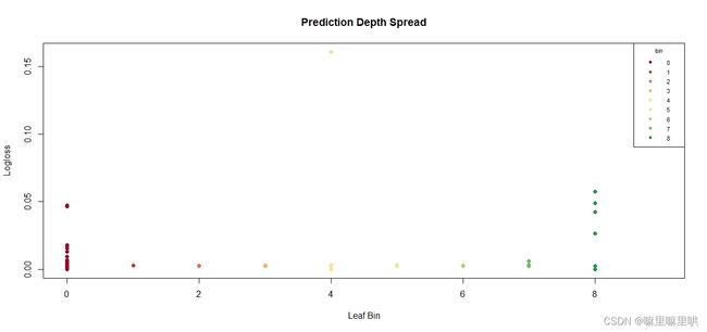
> .prediction_depth_spread_plot <- function(df) {
+ plot(
+ x = df$binned
+ , xlim = c(0L, 9L)
+ , y = df$Z
+ , type = "p"
+ , main = "Prediction Depth Spread"
+ , xlab = "Leaf Bin"
+ , ylab = "Logloss"
+ , pch = 19L
+ , col = .diverging_palette[df$binned + 1L]
+ )
+ legend(
+ "topright"
+ , title = "bin"
+ , legend = sort(unique(df$binned))
+ , pch = 19L
+ , col = .diverging_palette[sort(unique(df$binned + 1L))]
+ , cex = 0.7
+ )
+ }
>
> .depth_density_plot <- function(df) {
+ plot(
+ x = density(df$Y)
+ , xlim = c(min(df$Y), max(df$Y))
+ , type = "p"
+ , main = "Depth Density"
+ , xlab = "Prediction Probability"
+ , ylab = "Bin Density"
+ , pch = 19L
+ , col = .diverging_palette[df$binned + 1L]
+ )
+ legend(
+ "topright"
+ , title = "bin"
+ , legend = sort(unique(df$binned))
+ , pch = 19L
+ , col = .diverging_palette[sort(unique(df$binned + 1L))]
+ , cex = 0.7
+ )
+ }
备注:可视化每个样本下分箱的数量与预测值、log 损失之间的关系。
params <- list(objective = "regression", metric = "l2")
valids <- list(test = dtest)
model <- lgb.train(
    params
    , dtrain
    , 50L
    , valids
    , min_data = 1L
    , learning_rate = 0.1
    , bagging_fraction = 0.1
    , bagging_freq = 1L
    , bagging_seed = 1L
)
new_data <- data.frame(
    X = rowMeans(predict(
        model
        , agaricus.test$data
        , predleaf = TRUE
    )) # 预测了每棵树上叶子节点的索引
    , Y = pmin(
        pmax(
            predict(model, agaricus.test$data) # 回归问题的预测值
            , 1e-15
        )
        , 1.0 - 1e-15
    )
)
new_data$Z <- -1.0 * (agaricus.test$label * log(new_data$Y) + (1L - agaricus.test$label) * log(1L - new_data$Y)) # log loss

new_data$binned <- .bincode(
    x = new_data$X
    , breaks = quantile(
        x = new_data$X
        , probs = seq_len(9L) / 10.0
    )
    , right = TRUE
    , include.lowest = TRUE
)
new_data$binned[is.na(new_data$binned)] <- 0L
.prediction_depth_plot(df = new_data)
.prediction_depth_spread_plot(df = new_data)
.depth_density_plot(df = new_data)


多分类问题
备注:使用
lightgbm对鸢尾花数据进行分类.
> iris$Species <- as.numeric(as.factor(iris$Species)) - 1L
> train <- as.matrix(iris[c(1L:40L, 51L:90L, 101L:140L), ])
> test <- as.matrix(iris[c(41L:50L, 91L:100L, 141L:150L), ])
> dtrain <- lgb.Dataset(data = train[, 1L:4L], label = train[, 5L])
> dtest <- lgb.Dataset.create.valid(dtrain, data = test[, 1L:4L], label = test[, 5L])
> valids <- list(test = dtest)
>
>
> params <- list(objective = "multiclass", metric = "multi_error", num_class = 3L)
> model <- lgb.train(
+     params
+     , dtrain
+     , 100L
+     , valids
+     , min_data = 1L
+     , learning_rate = 1.0
+     , early_stopping_rounds = 10L
+ )
> my_preds <- predict(model, test[, 1L:4L]) # 返回向量
> my_preds <- predict(model, test[, 1L:4L], reshape = TRUE) # num_data * num_class Matrix
样本权重
> weights1 <- rep(1.0 / 100000.0, 6513L)
> weights2 <- rep(1.0 / 100000.0, 1611L)
> data(agaricus.train, package = "lightgbm")
> train <- agaricus.train
> dtrain <- lgb.Dataset(train$data, label = train$label, weight = weights1)
> data(agaricus.test, package = "lightgbm")
> test <- agaricus.test
> dtest <- lgb.Dataset.create.valid(dtrain, test$data, label = test$label, weight = weights2)
> valids <- list(test = dtest)
> params <- list(
+     objective = "regression"
+     , metric = "l2"
+     , device = "cpu"
+     , min_sum_hessian = 10.0
+     , num_leaves = 7L
+     , max_depth = 3L
+     , nthread = 1L
+ )
> model <- lgb.train(
+     params
+     , dtrain
+     , 50L
+     , valids
+     , min_data = 1L
+     , learning_rate = 1.0
+     , early_stopping_rounds = 10L
+ )
> weight_loss <- as.numeric(model$record_evals$test$l2$eval)
>
> plot(weight_loss) # Shows how poor the learning was: a straight line!
> params <- list(
+     objective = "regression"
+     , metric = "l2"
+     , device = "cpu"
+     , min_sum_hessian = 1e-4
+     , num_leaves = 7L
+     , max_depth = 3L
+     , nthread = 1L
+ )
> model <- lgb.train(
+     params
+     , dtrain
+     , 50L
+     , valids
+     , min_data = 1L
+     , learning_rate = 1.0
+     , early_stopping_rounds = 10L
+ )
> small_weight_loss <- as.numeric(model$record_evals$test$l2$eval)

总结:关于
lightgbm的使用教程就到此为止,如果博客中有没有说明白的地方,欢迎大家评论区提问。