1 The Machine Learning Landscape
1. The Machine Learning Landscape
Click here for notes and code
What Is Machine Learning?
- [Machine Learning is the] field of study that gives computers the ability to learn without being explicitly programmed.—Arthur Samuel, 1959
- A computer program is said to learn from experience E with respect to some task T and some performance measure P, if its performance on T, as measured by P, improves with experience E. —Tom Mitchell, 1997
An Example: spam filter
Learn to flag spam given examples of spam emails and examples of regular emails.
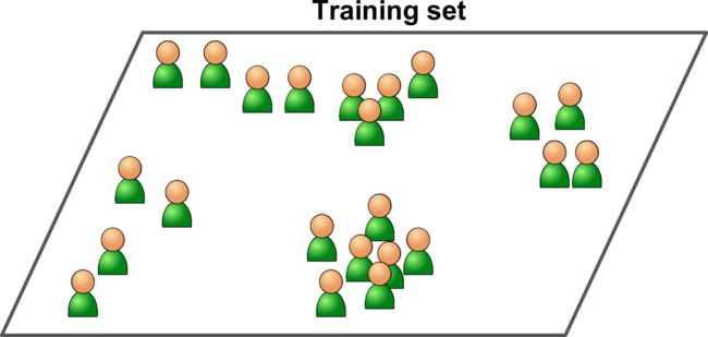
- Examples → Training set
- Each training example → Training instance(sample)
- The task T → Flag spam for new emails
- The experience E → The training data
- The performance measure P → ?
- Need to be define
- accuracy: The ratio of correctly classified emails
Why Use Machine Learning?
-
Use traditional programming techniques → A long list of complex rules—pretty hard to maintain
-
Use Machine Learning techniques → A spam filter automatically ****learns which words and phrases are good predictors of spam by detecting unusually frequent patterns of words in the spam examples compared to the ham examples.
- If spammers notice that all their emails containing “4U” are blocked, theymight start writing “For U” instead. A spam filter using traditional programming techniques would need to be updated to flag “For U” emails.
- A spam filter based on Machine Learning techniques automatically notices that “For U” has become unusually frequent in spam flagged by users.
Machine Learning is great for:
- Problems for which existing solutions require a lot of hand-tuning or long lists of rules: one Machine Learning algorithm can often simplify code and perform better.
- Complex problems for which there is no good solution at all using a traditional approach: the best Machine Learning techniques can find a solution.
- Fluctuating environments: a Machine Learning system can adapt to new data.
- Getting insights about complex problems and large amounts of data.
Formulization of the Example
- Input: x ∈ R d \boldsymbol{x}\in \mathbb{R}^d x∈Rd
- Email Feature
- Output: y , y i = { 0 , 1 } \boldsymbol{y},y_i = \{0,1\} y,yi={0,1}
- Email Classes : 0 for Not-spam and 1 for Spam
- Data: ( x 1 , y 1 ) , . . . , ( x n , y n ) (\boldsymbol{x}_1,y_1),...,(\boldsymbol{x}_n,y_n) (x1,y1),...,(xn,yn)
- Dataset of Spam/Not-Spam emails
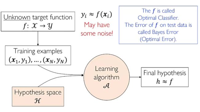
- Target function: f : x → y f:\boldsymbol{x}\rightarrow \boldsymbol{y} f:x→y
- Ideal Spam Filter → \rightarrow → unknown
Training to find a hypothesis……
- Hypothesis: h : x → y h:\boldsymbol{x}\rightarrow \boldsymbol{y} h:x→y
- Formula to be used for prediction
- It’s possible that f and h are not the same function
The two core components of the learning problem:
- The hypothesis space
H = { h } \mathcal{H}=\{h\} H={h}
h ∈ H h∈\mathcal{H} h∈H - The learning algorithm A \mathcal{A} A
- To find the best h
- They are together referred to as the learning model
Hypothesis Space
-
A hypothesis space H \mathcal{H} H is a set of functions that maps x → y x\rightarrow y x→y.
- It is the collection of prediction functions we are choosing from.
-
We want hypothesis space that…
- Includes only those functions that have desired regularity
- Continuity
- Smoothness
- Simplicity
- • Easy to work with
- Includes only those functions that have desired regularity
-
An example hypothesis space:
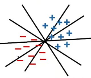
- All linear hyperplanes for classification→How to find the best?
- All hyperplanes in two dimensions are a hypothetical space. The learning algorithm finds the best hyperplane from this hypothesis space to maximize the divisibility of the data.
Loss Funcion
-
Loss function: l : y × y → R + l:y\times y\rightarrow \mathbb{R}_+ l:y×y→R+ measures the difference between h ( x ) h(x) h(x) and y y y
l ( y , h ( x ) ) = ( y − h ( x ) ) 2 (Regressison) l ( y , h ( x ) ) = 1 [ y ≠ h ( x ) ] (Classification) l(y,h(x))=(y-h(x))^2 \text{(Regressison)}\\l(y,h(x))=1[y \neq h(x)] \text{(Classification)} l(y,h(x))=(y−h(x))2(Regressison)l(y,h(x))=1[y=h(x)](Classification)
-
The canonical training procedure of machine learning:
Error of training:
ϵ ^ ( h ) = min ∑ i = 1 m l ( h θ ( x i ) , y i ) \hat\epsilon(h)=\min{\sum_{i=1}^m}l(h_\theta(x_i),y_i) ϵ^(h)=mini=1∑ml(hθ(xi),yi)
- Fit dataset with best hypothesis
- θ \theta θ is parameters of the hypothesis h h h
-
Virtually every machine learning algorithm has this form, just specify
- What is the hypothesis function?
- What is the loss function?
- How do we solve the training problem?
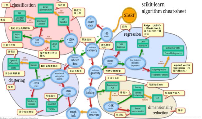
Types of Machine Learning Systems
Supervised/Unsupervised Learning
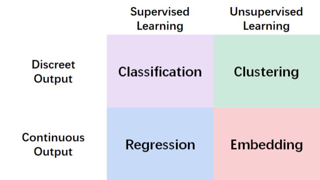
Supervised learning
In supervised learning, the training data you feed to the algorithm includes the desired
solutions, called labels.
-
classification
-
regression
Here are some of the most important supervised learning algorithms:
- k-Nearest Neighbors
- Linear Regression
- Logistic Regression
- Support Vector Machines (SVMs)
- Decision Trees and Random Forests
- Neural networks
Unsupervised learning
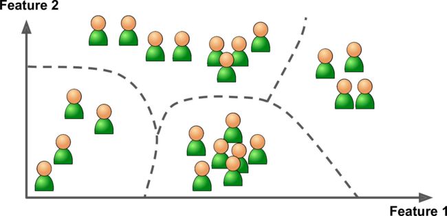
In unsupervised learning, as you might guess, the training data is unlabeled. The system tries to learn without a teacher.
Here are some of the most important unsupervised learning algorithms:
- Clustering
- K-Means
- DBSCAN
- Hierarchical Cluster Analysis (HCA)
- Anomaly detection and novelty detection
- One-class SVM
- Isolation Forest
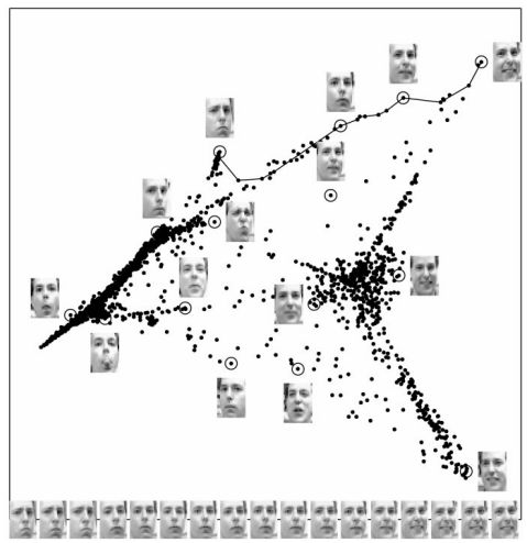
- Visualization and dimensionality reduction
- Principal Component Analysis (PCA)
- Kernel PCA
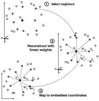
- Locally-Linear Embedding (LLE)
- t-distributed Stochastic Neighbor Embedding (t-SNE)
- Association rule learning
- Apriori
- Eclat
Semisupervised learning
Some algorithms can deal with partially labeled training data, usually a lot of unlabeled data and a little bit of labeled data. This is called semisupervised learning.
An Example: Google Photo
Reinforcement Learning
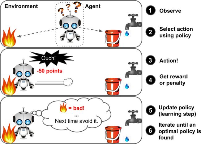
Reinforcement Learning is a very different beast. The learning system, called an agent in this context, can observe the environment, select and perform actions, and get rewards in return.
Main Challenges of Machine Learning
- bad data
- bad algorithm
Insufficient Quantity of Training Data
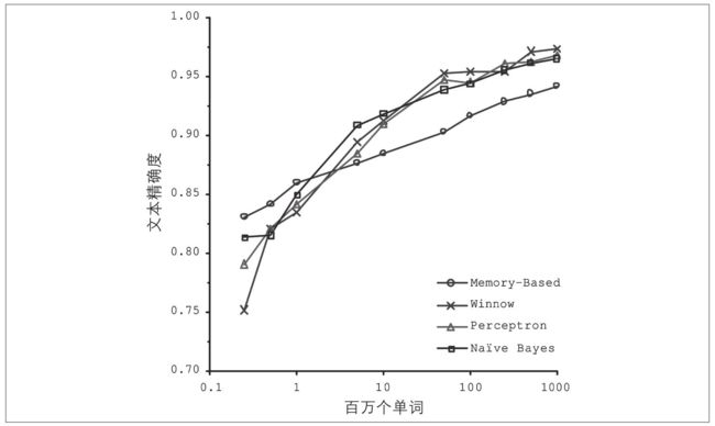
Microsoft researchers have shown that, given enough data, radically different machine learning algorithms (including fairly simple ones) can perform almost exactly the same job on the complex problem of natural language ambiguity reduction.
As the authors put it: “these results suggest that we may want to reconsider the tradeoff between spending time and money on algorithm development versus spending it
on corpus development.”
Small- and mediumsized datasets are still very common, and it is not always easy or cheap to get extra training data, so don’t abandon algorithms.
Nonrepresentative Training Data
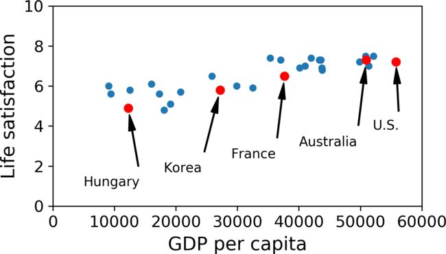
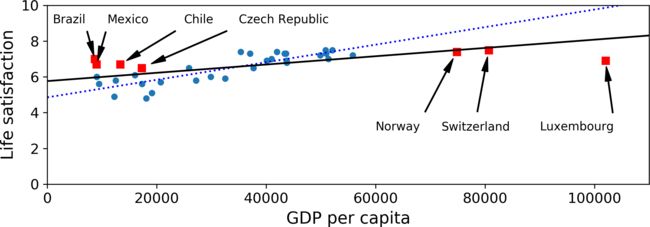
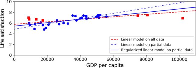
For example, when the GDP per capita-Life satisfaction line is fitted, when the data of some countries is missing and when the complete data is added, the line fitted is different.
- By using a nonrepresentative training set, we trained a model that is unlikely to make
accurate predictions, especially for very poor and very rich countries. - It is crucial to use a training set that is representative of the cases you want to generalize to.
- If the sample is too small, you will have sampling noise , but even very large samples can be nonrepresentative if the sampling method is flawed. This is called sampling bias.
Poor-Quality Data
If the training data is full of errors, outliers, and noise, it will make it harder for the system is less likely to perform well. It is often well worth the effort to spend time cleaning up your training data.
- some instances are clearly outliers
- simply discard them
- try to fix the errors manually.
- some instances are missing a few features (e.g., 5% of your customers did not specify their age)
- ignore this attribute altogether
- ignore these instances
- fill in the missing values (e.g., with the medianage)
- train one model with the feature and one model without it, and so on.
Irrelevant Features
A critical part of the success of a Machine Learning project is coming up with a good set of features to train on. This process, called feature engineering, involves:
- Feature selection: selecting the most useful features to train on among existing features.
- Feature extraction: combining existing features to produce a more useful one (like dimensionality reduction algorithms).
- Creating new features by gathering new data.
Overtting the Training Data
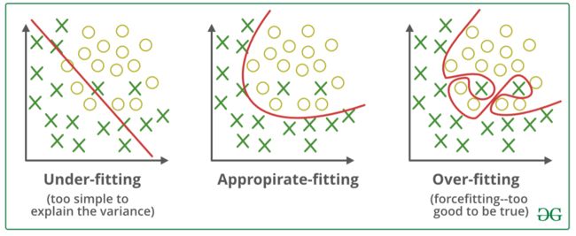
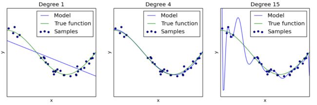
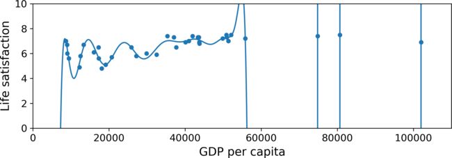
The below figure shows an example of a high-degree polynomial life satisfaction model that strongly overfits the training data. Even though it performs much better on the training data than the simple linear model, we cannot trust its predictions.
Overfitting happens when the model is too complex relative to the amount and noisiness of the training data. The possible solutions are:
- To simplify the model by selecting one with fewer parameters
- To gather more training data
- To reduce the noise in the training data (e.g., fix data errors and remove outliers)
Constraining a model to make it simpler and reduce the risk of overfitting is called regularization.
For example, the linear model we defined earlier has two parameters, θ 0 θ_0 θ0 and θ 1 θ_1 θ1.
- This gives the learning algorithm two degrees of freedom to adapt the model to the training data:
- If we forced θ 1 θ_1 θ1, the algorithm would have only one degree of freedom and would have a much harder time fitting the data properly. All it could do is move the line up or down to get as close as possible to the training instances, so it would end up around the mean.
- If we force it to keep it small, then the learning algorithm will effectively have somewhere in between one and two degrees of freedom. It will produce a simpler model than with two degrees of freedom, but more complex than with just one.
- We need to find the right balance between fitting the training data perfectly and keeping the model simple enough to ensure that it will generalize well.
In the same example of GDP above, we used the data of some missing countries for fitting, but regularization was added this time to get the blue solid line.
We can see that regularization forced the model to have a smaller slope, which fits a bit less the training data that the model was trained on, but actually allows it to generalize better to new examples.
The amount of regularization to apply during learning can be controlled by a hyperparameter.
- A hyperparameter is a parameter of a learning algorithm (not of the model).
- It is not affected by the learning algorithm itself;
- It must be set prior to training and remains constant during training.
- If you set the regularization hyper‐parameter to a very large value, you will get an almost flat model (a slope close to zero); the learning algorithm will almost certainly not overfit the training data, but it will be less likely to find a good solution.
- Tuning hyperparameters is an important part of building a Machine Learning system.
Undertting the Training Data
Underftting is the opposite of overfitting: it occurs when your model is too simple to learn the underlying structure of the data.
The main options to fix this problem are:
- Selecting a more powerful model, with more parameters
- Feeding better features to the learning algorithm (feature engineering)
- Reducing the constraints on the model (e.g., reducing the regularization hyperparameter)
Testing and Validating
The only way to know how well a model will generalize to new cases is to actually try it out on new cases.
A better option is to split your data into two sets: the training set and the test set.
- Train the parameters θ \theta θ of each model from the training data.
- Evaluate on the test data, and pick the best performer.
- The error rate on new cases is called the generalization error(or out-of-sample error), and by evaluating your model on the test set, you get an estimate of this error.
- If the training error is low (i.e., your model makes few mistakes on the training set)but the generalization error is high, it means that your model is overfitting the train‐ing data.
- The learning algorithms should never ever have access to test data!
- Problems:
-
Over-estimates the test performance ("lucky"model)
This is the most common but wrong practice of machine learning.
-
⛳It is common to use 80% of the data for training and hold out 20% for testing.
Reserve some data for validation
- Train the parameters θ \theta θ of each model from the training data.
- Evaluate on the validation data, and pick the best performer.
- Reserve test data to benchmark the chosen model.
- Problems:
- Wasteful of training data (learning cannot use validation data).
- May bias the selection towards overly simple models.
- The learning algorithms should never ever have access to test data!
- Programming
-
Random sampling
Scikit-Learn provides a few functions to split datasets into multiple subsets in various ways. The simplest function is
train_test_split.[document]
sklearn.model_selection.**train_test_split**(**arrays*, *test_size=None*, *train_size=None*, *random_state=None*, *shuffle=True*, *stratify=None*)| Parameters: | *arrays: sequence of indexables with same length / shape[0]
Allowed inputs are lists, numpy arrays, scipy-sparse matrices or pandas dataframes. |
| — | — |
| | test_size: float or int, default=None
between 0.0 and 1.0 |
| | train_size: float or int, default=None
between 0.0 and 1.0 |
| | random_state: int, RandomState instance or None, default=None |
| Returns: | splitting: list, length=2 * len(arrays) |Examples
>>> import numpy as np >>> from sklearn.model_selection import train_test_split >>> X, y = np.arange(10).reshape((5, 2)), range(5) >>> X array([[0, 1], [2, 3], [4, 5], [6, 7], [8, 9]]) >>> list(y) [0, 1, 2, 3, 4] >>> X_train, X_test, y_train, y_test = train_test_split( ... X, y, test_size=0.33, random_state=42) ... >>> X_train array([[4, 5], [0, 1], [6, 7]]) >>> y_train [2, 0, 3] >>> X_test array([[2, 3], [8, 9]]) >>> y_test [1, 4] >>> train_test_split(y, shuffle=False) [[0, 1, 2], [3, 4]] -
Stratified sampling
The following code uses the
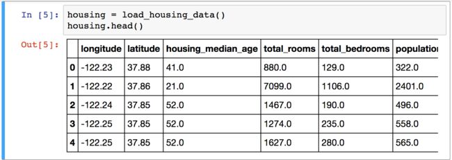
pd.cut()function to create an income category attribute with 5 categories (labeled from 1 to 5): category 1 ranges from 0 to 1.5 (i.e., less than $15,000), category 2 from1.5 to 3, and so on:housing["income_cat"] = pd.cut(housing["median_income"], bins=[0., 1.5, 3.0, 4.5, 6., np.inf], labels=[1, 2, 3, 4, 5]) housing["income_cat"].hist()Now you are ready to do stratified sampling based on the income category. For this
you can use Scikit-Learn’sStratifiedShuffleSplitclass:from sklearn.model_selection import StratifiedShuffleSplit split = StratifiedShuffleSplit(n_splits=1, test_size=0.2, random_state=42) for train_index, test_index in split.split(housing, housing["income_cat"]): strat_train_set = housing.loc[train_index] strat_test_set = housing.loc[test_index]Let’s see if this worked as expected. You can start by looking at the income category proportions in the test set:
>>> strat_test_set["income_cat"].value_counts() / len(strat_test_set)
3 0.350533
2 0.318798
4 0.176357
5 0.114583
1 0.039729
Name: income_cat, dtype: float64
Now you should remove the income_cat attribute so the data is back to its original
state:for set_ in (strat_train_set, strat_test_set): set_.drop("income_cat", axis=1, inplace=True)
-
K-fold Cross Validation
What if we get an unfortunate split?
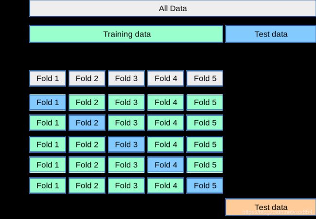
- Split the data set D \mathcal{D} D into K K K subset D ( i ) \mathcal{D^{(i)}} D(i)(called folds)
- For i = 1 , . . . , K i=1,...,K i=1,...,K, train h ( i ) h^{(i)} h(i) using all data but the i i i-th fold
- Cross-validation error by averaging all validation error ϵ ^ D ( i ) ( h ( i ) ) \hat\epsilon_{D^{(i)}}(h^{(i)}) ϵ^D(i)(h(i))
- In practice,we always choose K as 5 or 10.
- If we choose K K K as N N N (the size of D \mathcal{D} D), we get Leave-One-Out Cross
Validation (LOOCV)-only for small data, too costly for big data.
Model Seiection: Whole Procedure
Combined Algorithm Selection Hyperparameter (CASH)
optimization problem
-
A set of algorithms A = A ( 1 ) , . . . , A ( n ) \mathcal{A}={{A}^{(1)},...,{A}^{(n)}} A=A(1),...,A(n)
-
Denote the hyperparameter space of algorithm A ( i ) {A}^{(i)} A(i)as Λ ( i ) {\Lambda}^{(i)} Λ(i)
-
Denote the error of A ( i ) \mathcal{A}^{(i)} A(i) as L ( A λ ( i ) , D t r a i n , D v a l i d ) \mathcal{L}(A_\lambda^{(i)},D_{\rm train},D_{\rm valid}) L(Aλ(i),Dtrain,Dvalid) using λ ∈ Λ ( i ) \lambda \in \Lambda^{(i)} λ∈Λ(i) trained on D t r a i n D_{\rm train} Dtrain and evaluated on D v a l i d D_{\rm valid} Dvalid
-
The problem is to find optimal algorithm and its hyperparameter:
A λ ∗ ∗ = argmin A ( i ) ∈ A , λ ∈ Λ ( i ) L ( A λ ( i ) , D train , D valid ) A_{\lambda^*}^*=\underset{A^{(i)} \in \mathcal{A}, \lambda \in \boldsymbol{\Lambda}^{(i)}}{\operatorname{argmin}} \mathcal{L}\left(A_\lambda^{(i)}, D_{\text {train }}, D_{\text {valid }}\right) Aλ∗∗=A(i)∈A,λ∈Λ(i)argminL(Aλ(i),Dtrain ,Dvalid )
Complexity = ∑ A ( i ) ∈ A ∣ Λ ( i ) ∣ ⋅ K ⋅ O ( A ( i ) ) \text { Complexity }=\sum_{A^{(i)} \in \mathcal{A}}\left|\boldsymbol{\Lambda}^{(i)}\right| \cdot K \cdot O\left(A^{(i)}\right) Complexity =A(i)∈A∑ Λ(i) ⋅K⋅O(A(i))


