4 Linear Model

4. Linear Model

Click here for notes and code

Linear Regression

An Example: Electricity Prediction

• Problem:Predict the peak power consumption in summer.

  Date	High Temperature(F)	Peak Demand(GW)
  2011-06-01	84.0	2.651
  2011-06-02	73.0	2.081
  2011-06-03	75.2	1.844
  …	…	…

• Feature Engineering:

  • Primary key cannot be used as the features.
  • Instance Space: High Temperature(F)
  • Label Space: Peak Demand(GW)

• How to map from X to y?

  • Exploratory Data Analysis(EDA)to ease model selection: EDA

    [外链图片转存失败,源站可能有防盗链机制,建议将图片保存下来直接上传(img-QCPd3h2J-1671689314032)(https://typora-1309501826.cos.ap-nanjing.myqcloud.com//%E6%9C%BA%E5%99%A8%E5%AD%A6%E4%B9%A0/image-20221213192518896.png)]

    • Why different peak demands for the same high temperature?

      It is inaccurate when using only one feature for prediction.

Linear Regression: Hypothesis Space

• Training data: $({\mathbf{x}}_1,y_1),({\mathbf{x}}_2,y_2),...,({\mathbf{x}}_{\mathbf{n}},y_n)$

  • Feature vector: $\mathbf{x}\in {\mathbb{R}}^d$, response: $y\in \mathbb{R}$

• Add a constant dimension to feature vector x:

  x = ( 1 x 1 ⋯ x d ) ∈ R d + 1 \boldsymbol{x}=\left(\begin{array}{c} 1 \\ \boldsymbol{x_1} \\ \cdots \\ \boldsymbol{x_d} \end{array}\right) \in \mathbb{R}^{d+1} x= ​1x1​⋯xd​​ ​∈Rd+1

• Prediction of hypothesis $h$ parametrized by $\mathbf{\theta }$

  $$h_{\mathbf{\theta }}(\mathbf{x})={\mathbf{\theta }}_0+\sum _{j=1}^a{\mathbf{\theta }}_{\mathbf{j}}{\mathbf{x}}_{\mathbf{j}}=\sum _{j=0}^a{\mathbf{\theta }}_{\mathbf{j}}{\mathbf{x}}_{\mathbf{j}}=\mathbf{\theta }\cdot \mathbf{x}$$

  • $\mathbf{\theta }$ is the model’s parameter vector, containing the bias term and the feature weights ${\mathbf{\theta }}_0$ to ${\mathbf{\theta }}_n$.
  • $\mathbf{x}$ is the instance’s feature vector, containing ${\mathbf{x}}_0$ to ${\mathbf{x}}_0$, with ${\mathbf{x}}_0$ always equal to 1.
  • $\ast \ast h_{\mathbf{\theta }}(\mathbf{x})$** is the hypothesis function, using the model parameters $\mathbf{\theta }$

  In Machine Learning, vectors are often represented as column vectors, which are 2D arrays with a single column.
  If $\ast \ast \mathbf{\theta }\ast \ast$ and $\ast \ast \mathbf{x}\ast \ast$ are column vectors, then the prediction is: $\ast \hat{y}={\mathbf{\theta }}^T\mathbf{x}\ast$

Linear Regression: Loss Function

• Use the squared loss (L2 loss) to compute the error on training set

  $$\widehat{ϵ}(h)=\sum _{i=1}^n{\left(h\left({\mathbf{x}}_i\right)-y_i\right)}^2$$

  Or the Mean Square Error (MSE)

  $$\mathrm{MSE}\left(\mathbf{X},h_{\mathbf{\theta }}\right)=\frac{1}{m}\sum _{i=1}^m{\left({\mathbf{\theta }}^T{\mathbf{x}}_i-y_i\right)}^2$$

  To simplify notations, we will just write $\text{MSE}(\mathbf{\theta })$ instead of $\text{MSE}(\mathbf{X},\mathbf{\theta })$

  [外链图片转存失败,源站可能有防盗链机制,建议将图片保存下来直接上传(img-uxGuSmrm-1671689314033)(https://typora-1309501826.cos.ap-nanjing.myqcloud.com//%E6%9C%BA%E5%99%A8%E5%AD%A6%E4%B9%A0/image-20221213194217778.png)]

Linear Regression: Analytical Solution

[外链图片转存失败,源站可能有防盗链机制,建议将图片保存下来直接上传(img-lzz3MyjU-1671689314033)(https://typora-1309501826.cos.ap-nanjing.myqcloud.com//%E6%9C%BA%E5%99%A8%E5%AD%A6%E4%B9%A0/image-20221213200243725.png)]

Optimization

$$\underset{\mathbf{\theta }}{\min }\sum _{i=1}^n{\left(h_{\mathbf{\theta }}\left({\mathbf{x}}_i\right)-y_i\right)}^2$$

• Training error of linear regression:

  $$\begin{array}{rl}\widehat{ϵ}(\mathbf{\theta })& =\sum _{i=1}^n{\left({\mathbf{\theta }}^T{\mathbf{x}}_i-y_i\right)}^2\\ & =\Vert X\mathbf{\theta }-y{\Vert }^2\end{array}$$

• Put everything in matrix form:

  data matrix(design matrix) n×(d+1)

  label matrix n

  X = [ − x 1 T − − x 2 T − ⋮ − x n T − ] , y = [ y 1 y 2 ⋮ y n ] \boldsymbol{X}=\left[\begin{array}{c}-\boldsymbol{x}_1^T- \\ -\boldsymbol{x}_2^T- \\ \vdots \\ -\boldsymbol{x}_n^T-\end{array}\right], \quad \boldsymbol{y}=\left[\begin{array}{c}y_1 \\ y_2 \\ \vdots \\ y_n\end{array}\right] X= ​−x1T​−−x2T​−⋮−xnT​−​ ​,y= ​y1​y2​⋮yn​​ ​

  Computing the gradient of $\mathbf{\theta }$ and setting it to zero yields the optimal parameter ${\mathbf{\theta }}^{\ast }$:

  $$\begin{array}{rl}\widehat{ϵ}(\mathbf{\theta })& =\Vert \mathbf{X}\mathbf{\theta }-\mathbf{y}{\Vert }^2\\ {\nabla }_{\mathbf{\theta }}\widehat{ϵ}(\mathbf{\theta })& =2{\mathbf{X}}^T(\mathbf{X}\mathbf{\theta }-\mathbf{y})=0\\ & \Rightarrow {\mathbf{X}}^T\mathbf{X}\mathbf{\theta }={\mathbf{X}}^T\mathbf{y}\\ & \Rightarrow \mathbf{\theta }={\left({\mathbf{X}}^T\mathbf{X}\right)}^{-1}{\mathbf{X}}^T\mathbf{y}\end{array}$$

  • Computational complexity is big! $O[d^2(d+n)]$

Let’s generate some linear-looking data to test this equation $\mathbf{\theta }={\left({\mathbf{X}}^T\mathbf{X}\right)}^{-1}{\mathbf{X}}^T\mathbf{y}$

import numpy as np

X = 2 * np.random.rand(100, 1)
y = 4 + 3 * X + np.random.randn(100, 1)

X_b = np.c_[np.ones((100, 1)), X] # add x0 = 1 to each instance
theta_best = np.linalg.inv(X_b.T.dot(X_b)).dot(X_b.T).dot(y)

>>> theta_best
array([[4.21509616],
			 [2.77011339]])

We would have hoped for $\ast {\theta }_0\ast$ = 4 and $\ast {\theta }_1\ast$ = 3 instead of $\ast {\theta }_0\ast$ = 4.215 and $\ast {\theta }_1\ast$ = 2.770. Close

enough, but the noise made it impossible to recover the exact parameters of the original function.

Now you can make predictions using $\ast \ast \hat{\mathbf{\theta }}\ast \ast$:

>>> X_new = np.array([[0], [2]])
>>> X_new_b = np.c_[np.ones((2, 1)), X_new] # add x0 = 1 to each instance
>>> y_predict = X_new_b.dot(theta_best)
>>> y_predict
array([[4.21509616],
 [9.75532293]])

Plot this model’s predictions

plt.plot(X_new, y_predict, "r-")
plt.plot(X, y, "b.")
plt.axis([0, 2, 0, 15])
plt.show()

Performing linear regression using Scikit-Learn is quite simple:

>>> from sklearn.linear_model import LinearRegression

>>> lin_reg = LinearRegression()
>>> lin_reg.fit(X, y)
>>> lin_reg.intercept_, lin_reg.coef_
(array([4.21509616]), array([[2.77011339]]))
>>> lin_reg.predict(X_new)
array([[4.21509616],
 [9.75532293]])

Now we will look at very different ways to train a Linear Regression model, better
suited for cases where there are a large number of features, or too many training
instances to fit in memory.

Optimization: Gradient Descent

For general differentiable loss function,use Gradient Descent(GD)

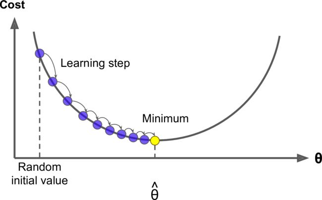
Concretely, you start by filling θ with random values (random initialization), and then you improve it gradually, taking one baby step at a time, each step attempting to decrease the cost function, until the algorithm converges to a minimum

• Gradient​

  • Gradient shows direction that function varies fastest

    $$\begin{array}{c}\mathbf{g}={\nabla }_{\mathbf{w}}J(\mathbf{w})\\ g_j={\nabla }_{w_j}J(\mathbf{w})\end{array}$$

[外链图片转存失败,源站可能有防盗链机制,建议将图片保存下来直接上传(img-5btkDVXN-1671689314034)(https://typora-1309501826.cos.ap-nanjing.myqcloud.com//%E6%9C%BA%E5%99%A8%E5%AD%A6%E4%B9%A0/tiduxiajiang-1.png)]

• Progress:

  • First-order Taylor approximation of the objective function:

    $$J(\mathbf{w})=J\left({\mathbf{w}}_0\right)+{\left(\mathbf{w}-{\mathbf{w}}_0\right)}^T\mathbf{g}+\cdots$$

  • Go along gradient for a step with a small rate $\eta$:

    An important parameter in Gradient Descent is the size of the steps, determined by the learning rate hyperparameter. If the learning rate is too small, then the algorithm will have to go through many iterations to converge, which will take a long time

  $$J(\mathbf{w}-\eta \mathbf{g})\approx J(\mathbf{w})-\eta {\mathbf{g}}^T\mathbf{g}$$

  

  

  • Repeat this step, and we get the Gradient Descent(GD) algorithm.

• Finally, not all cost functions are convex .There may be holes, ridges, plateaus, and all sorts of irregular terrains, making convergence to the minimum very difficult.

  The figure below shows the two main challenges with Gradient Descent: if the random initialization starts the algorithm on the left, then it will converge to a local minimum, which is not as good as the global minimum. If it starts on the right, then it will take a very long time to cross the plateau, and if you stop too early you will never reach the global minimum.

  

Fortunately, the MSE cost function for a Linear Regression model happens to be a convex function.

In fact, the cost function has the shape of a bowl, but it can be an elongated bowl if
the features have very different scales.

• On the left the Gradient Descent algorithm goes straight toward the minimum, thereby reaching it quickly,
• On the right it first goes in a direction almost orthogonal to the direction of the global minimum, and it ends with a long march down an almost flat valley. It will eventually reach the minimum, but it will take a long time.

When using Gradient Descent, you should ensure that all features have a similar scale (e.g., using Scikit-Learn’s StandardScaler class), or else it will take much longer to converge.

Batch Gradient Descent

• Partial derivatives of the cost function

  $$\frac{\partial }{\partial {\theta }_j}\mathrm{MSE}(\mathbf{\theta })=\frac{2}{m_i}\sum _{i=1}^m\left({\mathbf{\theta }}^T{\mathbf{x}}^{(i)}-y^{(i)}\right)x_j^{(i)}$$

• Gradient vector of the cost function

  ∇ θ MSE ⁡ ( θ ) = ( ∂ ∂ θ 0 MSE ⁡ ( θ ) ∂ ∂ θ 1 MSE ⁡ ( θ ) ⋮ ∂ ∂ θ n MSE ⁡ ( θ ) ) = 2 m X T ( X θ − y ) \nabla_{\boldsymbol{\theta}} \operatorname{MSE}(\boldsymbol{\theta})=\left(\begin{array}{c}\dfrac{\partial}{\partial \theta_0} \operatorname{MSE}(\boldsymbol{\theta}) \\\dfrac{\partial}{\partial \theta_1} \operatorname{MSE}(\boldsymbol{\theta}) \\\vdots \\\dfrac{\partial}{\partial \theta_n} \operatorname{MSE}(\boldsymbol{\theta})\end{array}\right)=\frac{2}{m} \mathbf{X}^T(\mathbf{X} \boldsymbol{\theta}-\mathbf{y}) ∇θ​MSE(θ)= ​∂θ0​∂​MSE(θ)∂θ1​∂​MSE(θ)⋮∂θn​∂​MSE(θ)​ ​=m2​XT(Xθ−y)

Once you have the gradient vector, which points uphill, just go in the opposite direction to go downhill.

$${\mathbf{\theta }}^{\text{(next step })}=\mathbf{\theta }-\eta {\nabla }_{\mathbf{\theta }}\mathrm{MSE}(\mathbf{\theta })$$

A quick implementation of this algorithm:

eta = 0.1 # learning rate
n_iterations = 1000
theta = np.random.randn(2,1) # random initialization
for iteration in range(n_iterations):
    gradients = 2/m * X_b.T.dot(X_b.dot(theta) - y)
    theta = theta - eta * gradients

>>> theta
array([[4.21509616],
 [2.77011339]])

The first 10 steps of Gradient Descent using three different learning rates.

• On the left, the learning rate is too low.
• In the middle, the learning rate looks pretty good.
• On the right, the learning rate is too high: the algorithm diverges, jumping all over the place and actually getting further and further away from the solution at every step.

How to set the number of iterations?

• A simple solution is to set a very large number of iterations but to interrupt the algorithm when the gradient vector becomes tiny—that is, when its norm becomes smaller than a tiny number ϵ (called the tolerance).

Stochastic Gradient Descent

Stochastic Gradient Descent just picks a random instance in the training set at every step and computes the gradients based only on that single instance.

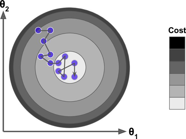
Due to its stochastic (i.e., random) nature, this algorithm is much less regular than Batch Gradient Descent: instead of gently decreasing until it reaches the minimum, the cost function will bounce up and down, decreasing only on average.

The final parameter values are good, but not optimal. When the cost function is very irregular , this can actually help the algorithm jump out of local minima, so Stochastic Gradient Descent has a better chance of finding the global minimum than Batch Gradient Descent does.

One solution to this dilemma is to gradually reduce the learning rate → simulated annealing

When using Stochastic Gradient Descent, the training instances must be independent and identically distributed (IID), to ensure that the parameters get pulled towards the global optimum, on average.
A simple way to ensure this is to shuffle the instances during training.

To perform Linear Regression using SGD the SGDRegressor class of Scikit-Learn, which defaults to optimizing the squared error cost function.

• Run for maximum 1000 epochs (max_iter=1000) or until the loss drops
  by less than 1e-3 during one epoch (tol=1e-3)
• Start with a learning rate of 0.1 (eta0=0.1)

from sklearn.linear_model import SGDRegressor

sgd_reg = SGDRegressor(max_iter=1000, tol=1e-3, penalty=None, eta0=0.1)
sgd_reg.fit(X, y.ravel())

>>> sgd_reg.intercept_, sgd_reg.coef_
(array([4.24365286]), array([2.8250878]))

Mini-batch Gradient Descent

Stochastic Gradient Descent: at each step, instead of computing the gradients based on the full training set (as in Batch GD) or based on just one instance (as in Stochastic GD), Mini batch GD computes the gradients on small random sets of instances called minibatches

Comparison of algorithms for Linear Regression:

Nonlinearization: Polynomial Regression

An Example: Electricity Prediction

• Problem: Predict the peak power consumption in all months.

• Exploratory Data Analysis(EDA): Peak demand vs.temperature plot

  [外链图片转存失败,源站可能有防盗链机制,建议将图片保存下来直接上传(img-ibavGyLk-1671689314036)(https://typora-1309501826.cos.ap-nanjing.myqcloud.com//%E6%9C%BA%E5%99%A8%E5%AD%A6%E4%B9%A0/image-20221214212320372.png)]

• Can we use linear regression again?

First, generate some nonlinear data, based on a simple quadratic equation

m = 100
X = 6 * np.random.rand(m, 1) - 3
y = 0.5 * X**2 + X + 2 + np.random.randn(m, 1)

let’s use Scikit-Learn’s PolynomialFeatures class to transform our training data, adding the square (2nd-degree polynomial) of each feature in the training set as new features:

>>> from sklearn.preprocessing import PolynomialFeatures
>>> poly_features = PolynomialFeatures(degree=2, include_bias=False)
>>> X_poly = poly_features.fit_transform(X)
>>> X[0]
array([-0.75275929])
>>> X_poly[0]
array([-0.75275929, 0.56664654])

>>> lin_reg = LinearRegression()
>>> lin_reg.fit(X_poly, y)
>>> lin_reg.intercept_, lin_reg.coef_
(array([1.78134581]), array([[0.93366893, 0.56456263]]))

Not bad: the model estimates $\hat{y}=0.56x_1^2+0.93x_1+1.78$ when in fact the original
function was $\hat{y}=0.5x_1^2+1.0x_1+2.0+\text{Guassian noise}$

Basis Function

• Feature map:

  $$\begin{array}{c}\mathbf{x}=\left(x_1,\dots ,x_d\right)\in \mathcal{X}\stackrel{\Phi }{⟶}\mathbf{z}=\left(z_1,\dots ,z_{\tilde{d}}\right)\in \mathcal{Z}\\ \mathbf{z}=\Phi (\mathbf{x})\end{array}$$

• Each $z_j={\varphi }_j(x)$ depends on some nonlinear transform ${\varphi }_j(x)$.

• $\{{\varphi }_j(x){\}}_{1\le j\le d}$ is called basis functions.

• Polynomial basis functions

  • 1-D vector: ${\mathbf{z}}^{\prime }=(1,x_1,x_1^2,x_1^3)$

    [外链图片转存失败,源站可能有防盗链机制,建议将图片保存下来直接上传(img-Iy0AvLZE-1671689314037)(https://typora-1309501826.cos.ap-nanjing.myqcloud.com//%E6%9C%BA%E5%99%A8%E5%AD%A6%E4%B9%A0/Figure1.4c.png)]

  • 2-D vector: ${\mathbf{z}}^{\prime }=(1,x_2,x_1{x}_2,x_1^2)$

• Radial basis functions (RBF)

  ϕ j ( x ) = { exp ⁡ ( − ∥ x − μ j ∥ 2 2 2 σ 2 ) : j = 1 , … , d ~ } \phi_j(\boldsymbol{x})=\left\{\exp \left(-\frac{\left\|\boldsymbol{x}-\boldsymbol{\mu}_j\right\|_2^2}{2 \sigma^2}\right): j=1, \ldots, \tilde{d}\right\} ϕj​(x)={exp(−2σ2 ​x−μj​ ​22​​):j=1,…,d~}

• The final hypothesis is linear in the feature space $\mathcal{Z}$.

• The final hypothesis is nonlinear in the input space $\mathcal{X}$

  $$h(\mathbf{x})=\mathbf{\theta }\cdot \mathbf{z}=\mathbf{\theta }\cdot \Phi (\mathbf{x})=\sum _{j=1}^{\tilde{d}}{\theta }_j{\varphi }_j(\mathbf{x})$$

[外链图片转存失败,源站可能有防盗链机制,建议将图片保存下来直接上传(img-uyBoCt9k-1671689314037)(https://typora-1309501826.cos.ap-nanjing.myqcloud.com//%E6%9C%BA%E5%99%A8%E5%AD%A6%E4%B9%A0/image-20221214221245638.png)]

Learning Curves

The fighure below applies a 300-degree polynomial model to the preceding training data, and compares the result with a pure linear model and a quadratic model (2nd-degree polynomial). Notice how the 300-degree polynomial model wiggles around to get as close as possible to the training instances.

• The high-degree Polynomial Regression model is severely overfitting the
  training data.
• The linear model is underfitting the training data.

How to judge the model is overfitting or underfitting the data?

• cross-validation

  • If a model performs well on the training data but generalizes poorly according to the cross-validation metrics, then your model is overfitting.
  • If it performs poorly on both, then it is underfitting.

• learning curves

  • To generate the plots, simply train the model several times on different sized subsets of the training set.

  from sklearn.metrics import mean_squared_error
  from sklearn.model_selection import train_test_split
  
  def plot_learning_curves(model, X, y):
      X_train, X_val, y_train, y_val = train_test_split(X, y, test_size=0.2)
      train_errors, val_errors = [], []
      for m in range(1, len(X_train)):
          model.fit(X_train[:m], y_train[:m])
          y_train_predict = model.predict(X_train[:m])
          y_val_predict = model.predict(X_val)
          train_errors.append(mean_squared_error(y_train[:m], y_train_predict))
          val_errors.append(mean_squared_error(y_val, y_val_predict))
      plt.plot(np.sqrt(train_errors), "r-+", linewidth=2, label="train")
      plt.plot(np.sqrt(val_errors), "b-", linewidth=3, label="val")
      plt.legend(labels=['train','val'])
      plt.xlabel('Train set size')
      plt.ylabel('RMSE')
  

  lin_reg = LinearRegression()
  plot_learning_curves(lin_reg, X, y)
  

  

  Train:

  • When there are just one or two instances in the training set, the model can fit them perfectly, which is why the curve starts at zero.
  • But as new instances are added to the training set, it becomes impossible for the model to fit the training data perectly, both because the data is noisy and because it is not linear at all.
  • So the error on the training data goes up until it reaches a plateau, at which point adding new instances to the training set doesn’t make the average error much better or worse.

  Val:

  • When the model is trained on very few training instances, it is incapable of generalizing properly, which is why the validation error is initially quite big.
  • Then as the model is shown more training examples, it learns and thus the validation error slowly goes down.
  • However, once again a straight line cannot do a good job modeling the data, so the error ends up at a plateau, very close to the other curve.

  These learning curves are typical of an underfitting model. Both curves have reached a plateau; they are close and fairly high.

  If your model is underfitting the training data, adding more training examples will not help. You need to use a more complex model or come up with better features.

  Now let’s look at the learning curves of a 10th-degree polynomial model on the same data.

  from sklearn.pipeline import Pipeline
  polynomial_regression = Pipeline([
   ("poly_features", PolynomialFeatures(degree=10, include_bias=False)),
   ("lin_reg", LinearRegression()),
   ])
  plot_learning_curves(polynomial_regression, X, y)
  

  • The error on the training data is much lower than with the Linear Regression model.

  • There is a gap between the curves.

    This means that the model performs significantly better on the training data than on the validation data, which is the hall mark of an overfitting model.

    However, if you used a much larger training set, the two curves would continue to get closer.

  One way to improve an overfitting model is to feed it more training data until the validation error reaches the training error.

Regularization

Overfitting

• Higher-order polynomial fits data better.
• But may fit noise!
• Also may cause very large coefficients.

[外链图片转存失败,源站可能有防盗链机制,建议将图片保存下来直接上传(img-Or7dPN8r-1671689314038)(https://typora-1309501826.cos.ap-nanjing.myqcloud.com//%E6%9C%BA%E5%99%A8%E5%AD%A6%E4%B9%A0/Figure1.4c.png)]

[外链图片转存失败,源站可能有防盗链机制,建议将图片保存下来直接上传(img-oLVCf5yH-1671689314038)(https://typora-1309501826.cos.ap-nanjing.myqcloud.com//%E6%9C%BA%E5%99%A8%E5%AD%A6%E4%B9%A0/Figure1.4d.png)]

[外链图片转存失败,源站可能有防盗链机制,建议将图片保存下来直接上传(img-3RU5O46e-1671689314038)(https://typora-1309501826.cos.ap-nanjing.myqcloud.com//%E6%9C%BA%E5%99%A8%E5%AD%A6%E4%B9%A0/Figure1.5.png)]

http://gaolei786.github.io/statistics/prml1.html

• How to control the model complexity?

  Solution:Control norm of $\theta$ !

A good way to reduce overfitting is to regularize the model (i.e., to constrain it): the fewer degrees of freedom it has, the harder it will be for it to overfit the data.

For example, a simple way to regularize a polynomial model is to reduce the number of polynomial degrees.

L2-Regularization

The L2-regularized linear regression (ridge regression) imposes L2-norm regularization trading off with a hyperparameter $\lambda >0$, This forces the learning algorithm to not only fit the data but also keep the model weights as small as possible

$$\mathbf{w}=\underset{\mathbf{w}\in {\mathbb{R}}^d}{\mathrm{argmin}}\sum _{i=1}^n{\left({\mathbf{w}}^T{\mathbf{x}}_i-y_i\right)}^2+\lambda \Vert \mathbf{w}{\Vert }_2^2$$

• The hyperparameter $\lambda$ controls how much you want to regularize the model.

  • If $\lambda =0$ then Ridge Regression is just Linear Regression.
  • If $\lambda$ **is very large, then all weights end up very close to zero and the result is a flat line going through the data’s mean.

• Compute the gradient and set it to zero

  $$\begin{array}{rl}{\nabla }_w\widehat{ϵ}(\mathbf{w})& =2{\mathbf{X}}^T(\mathbf{X}\mathbf{w}-\mathbf{y})+2\lambda \mathbf{w}=0\\ & \Rightarrow \left({\mathbf{X}}^T\mathbf{X}+\lambda I\right)\mathbf{w}={\mathbf{X}}^T\mathbf{y}\\ & \Rightarrow \mathbf{w}={\left({\mathbf{X}}^T\mathbf{X}+\lambda I\right)}^{-1}{\mathbf{X}}^T\mathbf{y}\end{array}$$

  Here is how to perform Ridge Regression with Scikit-Learn using a closed-form solution.

  >>> from sklearn.linear_model import Ridge
  >>> ridge_reg = Ridge(alpha=1, solver="cholesky")
  >>> ridge_reg.fit(X, y)
  >>> ridge_reg.predict([[1.5]])
  array([[1.55071465]])
  

• Or using Gradient Descent (GD):

  $$-w^{t+1}\leftarrow w^t-{\eta {\nabla }_w\widehat{ϵ}(w)|}_{w=w^t}$$

  
  >>> sgd_reg = SGDRegressor(penalty="l2")
  >>> sgd_reg.fit(X, y.ravel())
  >>> sgd_reg.predict([[1.5]])
  array([1.47012588])
  

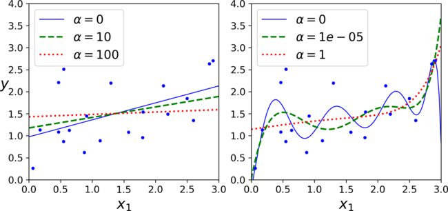
The figure below shows several Ridge models trained on some linear data using different α value. On the left, plain Ridge models are used, leading to linear predictions.

• On the left, plain Ridge models are used, leading to linear predictions.
• On the right, the data is first expanded using PolynomialFeatures(degree=10), then it is
  scaled using a StandardScaler, and the Ridge models are applied to the resulting features.

L1-Regularization

The L1-regularized linear regression (lasso regression) imposes L1-norm regularization trading off with a hyperparameter $\lambda \ge 0$:

$$\mathbf{w}=\underset{\mathbf{w}\in {\mathbb{R}}^d}{\mathrm{argmin}}\sum _{i=1}^n{\left({\mathbf{w}}^T{\mathbf{x}}_i-y_i\right)}^2+\lambda \Vert \mathbf{w}{\Vert }_1$$

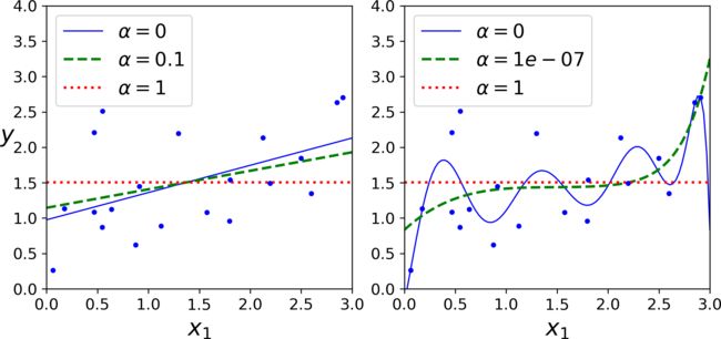
An important characteristic of Lasso Regression is that it tends to completely eliminate the weights of the least important features (i.e., set them to zero).

For example, the dashed line in the right plot on (with α = 10-7) looks quadratic, almost linear: all the weights for the high-degree polynomial features are equal to zero.

In other words, Lasso Regression automatically performs feature selection and outputs a

sparse model (i.e., with few nonzero feature weights).

The Lasso cost function is not differentiable at $\ast w_i=0\ast$ (for i = 1, 2, ⋯, n), but Gradient Descent still works fine if you use a subgradient vector $g$ ****15 instead when any $\ast w_i=0\ast$.

g ( w , J ) = ∇ w MSE ⁡ ( w ) + α ( sign ⁡ ( w 1 ) sign ⁡ ( w 2 ) ⋮ sign ⁡ ( w n ) )  where  sign ⁡ ( w i ) = { − 1  if  w i < 0 0  if  w i = 0 + 1  if  w i > 0 g(\boldsymbol{w}, J)=\nabla_{\boldsymbol{w}} \operatorname{MSE}(\boldsymbol{w})+\alpha\left(\begin{array}{c}\operatorname{sign}\left(w_1\right) \\\operatorname{sign}\left(w_2\right) \\\vdots \\\operatorname{sign}\left(w_n\right)\end{array}\right) \\\text { where }\operatorname{sign}\left(w_i\right)=\left\{\begin{array}{cc}-1 & \text { if } w_i<0 \\0 & \text { if } w_i=0 \\+1 & \text { if } w_i>0\end{array}\right. g(w,J)=∇w​MSE(w)+α ​sign(w1​)sign(w2​)⋮sign(wn​)​ ​ where sign(wi​)=⎩ ⎨ ⎧​−10+1​ if wi​<0 if wi​=0 if wi​>0​

Here is a small Scikit-Learn example using the Lasso class. Note that you could instead use an SGDRegressor(penalty="l1").

>>> from sklearn.linear_model import Lasso
>>> lasso_reg = Lasso(alpha=0.1)
>>> lasso_reg.fit(X, y)
>>> lasso_reg.predict([[1.5]])
array([1.53788174])

It is almost always preferable to have at least a little bit of regularization, so generally you should avoid plain Linear Regression.
Ridge is a good default, but if you suspect that only a few features are actually useful, you should prefer Lasso or Elastic Net since they tend to reduce the useless features’ weights down to zero as we have discussed.

Linear Classification

Logistic Regression

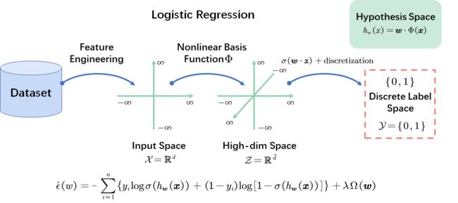
• How to design loss function over linear hypothesis for classification?
• Naive idea: $\underset{\mathbf{w}}{\min }\sum _{i=1}^n{\left(h_{\mathbf{w}}\left({\mathbf{x}}_i\right)-y_i\right)}^2+\lambda \Omega (\mathbf{w})$ where $y_i\in \{0,1\}$
  • Discretize the continuous output $h_{\mathbf{w}}$to be $\{0,1\}$
• During test part

• It does not make sense for $h_{\mathbf{w}}$ to take values larger than 1 or smaller than 0 when we know that $y\in \{0,1\}.$

• We use accuracy (01-loss)when validating the classification model:

  $$l(y,h(x))=1[y\ne h(x)]$$

  $h(\mathbf{x})\in y$ is not a proper assumption this time.

Logistic Regression:Link Function

Instead of outputting the result directly like the Linear Regression model does, it outputs the logistic of this result.

$$\hat{p}=h_{\mathbf{w}}(\mathbf{x})=\sigma ({\mathbf{x}}^T\mathbf{w})$$

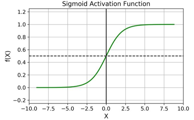
The logistic—noted σ(·)—is a sigmoid function (i.e., S-shaped) that outputs a number between 0 and 1.

$$\sigma (t)=\frac{1}{1+e^{-t}}$$

• Sigmoid maps $\mathbb{R}$ to $[0,1]$.
• $t\to +\infty ,\sigma (t)\to 1$
• Set $\sigma (h(\mathbf{x}))=p(y=1|x)$ as the probability to label $\mathbf{x}$ as $y=1$.

Logistic Regression:Loss Function

• How about using squared loss now as $h(\mathbf{x})\in [0,1]$ and $y\in \{0,1\}$？

  $$l(h(\mathbf{x}),y)=\sum _{i=1}^n{\left(\sigma \left({\mathbf{w}}^T{\mathbf{x}}_i\right)-y_i\right)}^2+\lambda \Omega (\mathbf{w})$$

  

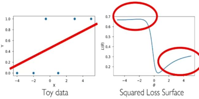
• Tries to match continuous probability with discrete 0/1 labels.

  • Non-convex
  • Small loss when prediction is overly far in wrong side
  • What is wrong?

Logistic Regression:Statistical View

• Under some proper distributional assumption:

  • The MLE of a parametric model leads to a particular loss function.

• Assume the conditional: $P(y=1\mid \mathbf{x},\mathbf{w})=\sigma \left({\mathbf{w}}^T\mathbf{x}\right)=\frac{1}{1+\exp \left(-{\mathbf{w}}^{T}x\right)}$

• Maximum Likelihood Estimation(MLE):

  $$\underset{\mathbf{w}}{\max }\prod _{i=1}^n\prod _{c=0}^{1}P{\left(y_i=c\mid {\mathbf{x}}_i,\mathbf{w}\right)}^{1\left\{y_i=c\right\}}$$

• Log-likelihood:

  $$-\frac{1}{n}\sum _{i=1}^n\sum _{c=0}^1\left\{1\left\{y_i=c\right\}\cdot \log P\left(y_i=c\mid {\mathbf{x}}_i\right)\right\}$$

• Derive the maximum log-likelihood estimation by plugging above in:

  $$\begin{array}{rl}& -\frac{1}{n}\sum _{i=1}^n\sum _{c=0}^1\left\{1\left\{y_i=c\right\}\cdot \log P\left(y_i=c\mid {\mathbf{x}}_i\right)\right\}\\ =& -\frac{1}{n}\sum _{i=1}^n\left\{y_i\log P\left(y_i=1\mid {\mathbf{x}}_i\right)+\left(1-y_i\right)\log P\left(y_i=0\mid {\mathbf{x}}_i\right)\right\}\\ =& -\frac{1}{n}\sum _{i=1}^n\{\underset{y_i}{y_i\log \sigma ({\mathbf{w}}^T{\mathbf{x}}_i})+\underset{y_i}{\left(1-y_i\right)\log [1-\sigma ({\mathbf{w}}^T{\mathbf{x}}_i})]\}\end{array}$$

Logistic Regression:Cross-Entropy Loss

$$\ell \left(h\left({\mathbf{x}}_i\right),y_i\right)=\{\begin{array}{ll}-\log \left[\sigma \left({\mathbf{w}}^T{\mathbf{x}}_i\right)\right]& y_i=1\\ -\log \left[1-\sigma \left({\mathbf{w}}^T{\mathbf{x}}_i\right)\right]& y_i=0\end{array}$$

• Check! If $y_i=1$

  • $\sigma \left({\mathbf{w}}^T{\mathbf{x}}_i\right)\to 0$, loss goes to $\infty$
  • $\sigma \left({\mathbf{w}}^T{\mathbf{x}}_i\right)\to 0$, loss goes to 0

  

• Logistic Regression cost function (log loss)

  $$\widehat{ϵ}(w)=-\sum _{i=1}^n\left\{y_i\log \sigma \left(h_{\mathbf{w}}(\mathbf{x})\right)+\left(1-y_i\right)\log \left[1-\sigma \left(h_{\mathbf{w}}(\mathbf{x})\right)\right]\right\}$$

Logistic Regression:Regularization

• A classification dataset is said to be linearly separable if there exists a hyperplane that separates the two classes.

  • Appears a lot in non-linear setting.

• If data is linearly separable after using nonlinear features, LR requires regularization.

• Prevent weights from diverging on linearly separable data

  $$\widehat{ϵ}(w)=-\sum _{i=1}^n\left\{y_i\log \sigma \left(h_{\mathbf{w}}(\mathbf{x})\right)+\left(1-y_i\right)\log \left[1-\sigma \left(h_{\mathbf{w}}(\mathbf{x})\right)\right]\right\}+\lambda \sum _{j=1}^a{w}_j^2$$

• Similar with regression:L1,L2…

  

• How to solve this problem?
  • The bad news is that there is no known closed-form equation to compute the value of w that minimizes this cost function (there is no equivalent of the Normal Equation). But the good news is that this cost function is convex, so Gradient Descent (or any other optimization algorithm) is guaranteed to find the global minimum (if the learning rate is not too large and you wait long enough).

Decision Boundaries

Let’s try to build a classifier to detect the Iris-Virginica type based only on the petal width feature. First let’s load the data:

>>> from sklearn import datasets
>>> iris = datasets.load_iris()
>>> list(iris.keys())
['data', 'target', 'target_names', 'DESCR', 'feature_names', 'filename']
>>> X = iris["data"][:, 3:] # petal width
>>> y = (iris["target"] == 2).astype(np.int) # 1 if Iris-Virginica, else 0

Now let’s train a Logistic Regression model:

from sklearn.linear_model import LogisticRegression
log_reg = LogisticRegression()
log_reg.fit(X, y)

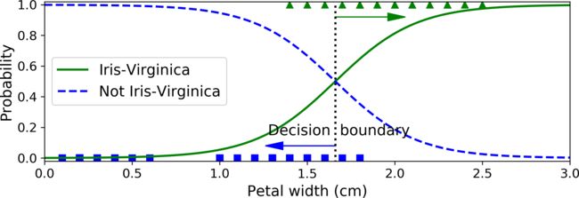
Let’s look at the model’s estimated probabilities for flowers with petal widths varying
from 0 to 3 cm:

X_new = np.linspace(0, 3, 1000).reshape(-1, 1)
y_proba = log_reg.predict_proba(X_new)
plt.plot(X_new, y_proba[:, 1], "g-", label="Iris-Virginica")
plt.plot(X_new, y_proba[:, 0], "b--", label="Not Iris-Virginica")

Above about 2 cm the classifier is highly confident that the flower is an IrisVirginica (it outputs a high probability to that class), while below 1 cm it is highly confident that it is not an Iris-Virginica (high probability for the “Not Iris-Virginica”class). In between these extremes, the classifier is unsure.

Softmax Regression

The Logistic Regression model can be generalized to support multiple classes directly, without having to train and combine multiple binary classifiers. This is called Softmax Regression, or Multinomial Logistic Regression.

Softmax Regression:Softmax Function

$$p(y=c\mid \mathbf{x};\mathbf{W})=\frac{\exp \left({\mathbf{w}}_c^T\mathbf{x}\right)}{{\sum }_{r=1}^C\exp \left({\mathbf{w}}_r^T\mathbf{x}\right)}$$

• $C$ is the number of classes.
• ${\mathbf{w}}_c^T\mathbf{x}$ is a vector containing the scores of each class for the instance x.
• $p$ is the estimated probability that the instance x belongs to class C **given the scores of each class for that instance.

Softmax Regression: Statistical View

• Categorical distribution assumption

  • Probability mass function:

    $$P(y=c\mid \mathbf{q})=q_c,\sum _{c=1}^C{q}_c=1$$

• Probability of flipping $m$ dices with result $\{y_1,...,y_m\}$

  $$\prod _{i=1}^m\prod _{c=1}^{c}P{\left(y_i=c\mid q_{ic}\right)}^{1\left\{y_i=c\right\}}$$

• Softmax regression assumes that given parameter $\mathbf{W}$:

  $$q_{ic}=P\left(y_i=c\mid x_{ij}W\right)$$

• The likelihood of $\mathbf{W}$ given all samples $\mathcal{D}=\left\{\left(\mathbf{x}i,y_i\right)\right\}{i=1}^m$

  $$\mathcal{L}(\mathbf{W};\mathcal{D})=\prod _{i=1}^m\prod _{c=1}^{c}P{\left(y_i=c\mid x_i;\mathbf{W}\right)}^{1\left\{y_i=c\right\}}$$

• Maximum likelihood estimation:

$$\mathcal{L}(\mathbf{W};\mathcal{D})=\underset{{\mathbf{w}}_1,\dots ,{\mathbf{w}}_{\mathcal{C}}}{\max }\prod _{i=1}^m\prod _{c=1}^{c}P{\left(y_i=c\mid x_i;\mathbf{W}\right)}^{1\left\{y_i=c\right\}}$$

• We use minimum negative log-likelihood estimation:

  $$\begin{array}{rl}& \mathcal{LL}(\mathbf{W};\mathcal{D})=\underset{{\mathbf{w}}_1,\dots ,{\mathbf{w}}_C}{\min }-\frac{1}{m}\sum _{i=1}^m\sum _{c=1}^c\left\{1\left\{y_i=c\right\}\cdot \log P\left(y_i=c\mid x_i;\mathbf{W}\right)\right\}\\ & =\underset{w_1,\dots ,w_C}{\min }-\frac{1}{m}\sum _{i=1}^m\sum _{c=1}^c\left\{1\left\{y_i=c\right\}\cdot \log \frac{\exp \left({\mathbf{w}}_c^T{\mathbf{x}}_i+{\mathbf{b}}_c\right)}{{\sum }_{r=1}^C\exp \left({\mathbf{w}}_r^T{\mathbf{x}}_i+{\mathbf{b}}_r\right)}\right\}\end{array}$$

Softmax Regression:Cross-Entropy Loss

$$-\frac{1}{m}\sum _{i=1}^m\sum _{c=1}^c\left\{1\left\{y_i=c\right\}\cdot \log \frac{\exp \left({\mathbf{w}}_c^T{\mathbf{x}}_i+{\mathbf{b}}_c\right)}{{\sum }_{r=1}^C\exp \left({\mathbf{w}}_r^T{\mathbf{x}}_i+{\mathbf{b}}_r\right)}\right\}$$

Let’s use Softmax Regression to classify the iris flowers into all three classes. ScikitLearn’s LogisticRegression uses one-versus-all by default when you train it on more than two classes, but you can set the multi_class hyperparameter to “multinomial” to switch it to Softmax Regression instead.You must also specify a solver that supports Softmax Regression, such as the “lbfgs” solver (see Scikit-Learn’s documentation for more details). It also applies ℓ2 regularization by default, which you can control using the hyperparameter C.

X = iris["data"][:, (2, 3)] # petal length, petal width
y = iris["target"]
softmax_reg = LogisticRegression(multi_class="multinomial",solver="lbfgs", C=10)
softmax_reg.fit(X, y)

>>> softmax_reg.predict([[5, 2]])
array([2])
>>> softmax_reg.predict_proba([[5, 2]])
array([[6.38014896e-07, 5.74929995e-02, 9.42506362e-01]])