12-TensorFlow RNN的简单使用
1.RNN概念
RNN: 借助循环核(cell)提取特征后,送入后续网络(如全连接网络 Dense) 进行预测等操作。RNN 借助循环核从时间维度提取信息,循环核参数时间共享。

1.循环核
循环核具有记忆力,通过不同时刻的参数共享,实现了对时间序列的信息提取。每个循环核有多个记忆体,对应图 1.2.1 中的多个小圆柱。记忆体内存储着每个时刻的状态信息ℎ,这里h = tanh( ℎ+ℎ−1wℎℎ + ℎ)。其中,ℎ、wℎℎ
为权重矩阵,ℎ为偏置,为当前时刻的输入特征,ℎ−1为记忆体上一时刻存储的状态信息,tanh 为激活函数。
当前时刻循环核的输出特征 = softmax(ℎℎ + y),其中ℎ为权重矩阵、y为偏置、softmax 为激活函数,其实就相当于一层全连接层。我们可以设定记忆体的个数从而改变记忆容量,当记忆体个数被指定、输入输出维度被指定,周围这些待训练参数的维度也就被限定了。在前向传播时,记忆体内存储的状态信息h在每个时刻都被刷新,而三个参数矩阵ℎ、wℎℎ、ℎ和两个偏置项ℎ、 y自始至终都是固定不变的。在反向传播时,三个参数矩阵和两个偏置项由梯度下降法更新。
2.循环核按时间步展开
将循环核按时间步展开,就是把循环核按照时间轴方向展开,可以得到如图1.2.2 的形式。每个时刻记忆体状态信息h被刷新,记忆体周围的参数矩阵和两个偏置项是固定不变的,我们训练优化的就是这些参数矩阵。训练完成后,使用效果最好的参数矩阵执行前向传播,然后输出预测结果。其实这和我们人类的预测是一致的:我们脑中的记忆体每个时刻都根据当前的输入而更新;当前的预测推理是根据我们以往的知识积累用固化下来的“参数矩阵”进行的推理判断。
可以看出,循环神经网络就是借助循环核实现时间特征提取后把提取到的信息送入全连接网络,从而实现连续数据的预测。

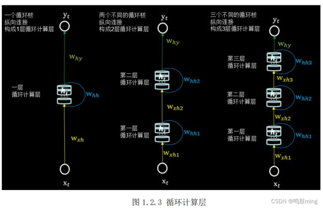
3.循环计算层:向输出方向生长
在 RNN 中,每个循环核构成一层循环计算层,循环计算层的层数是向输出方向增长的。如图 1.2.3 所示,左图的网络有一个循环核,构成了一层循环计算层;中图的网络有两个循环核,构成了两层循环计算层;右图的网络有三个循环核,
构成了三层循环计算层。其中,三个网络中每个循环核中记忆体的个数可以根据我们的需求任意指定。
4.RNN 训练
得到 RNN 的前向传播结果之后,和其他神经网络类似,我们会定义损失函数,使用反向传播梯度下降算法训练模型。RNN 唯一的区别在于:由于它每个时刻的节点都可能有一个输出,所以 RNN 的总损失为所有时刻(或部分时刻)上的损失和。
3.Tensorflow2 描述循环计算层
tf.keras.layers.SimpleRNN(神经元个数,activation=‘激活函数’,return_sequences=是否每个时刻输出ℎ到下一层)
(1)神经元个数:即循环核中记忆体的个数
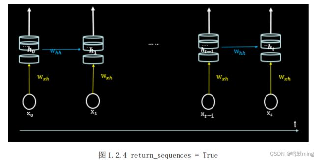
(2) return_sequences:在输出序列中,返回最后时间步的输出值ℎ还是返回全部时间步的输出。False 返回最后时刻(图 1.2.5),True 返回全部时刻(图1.2.4)。当下一层依然是 RNN 层,通常为 True,反之如果后面是 Dense 层,通常为 Fasle。

(3)输入维度:三维张量(输入样本数, 循环核时间展开步数, 每个时间步输入特征个数)。

如图 1.2.6 所示,左图一共要送入 RNN 层两组数据,每组数据经过一个时间步就会得到输出结果,每个时间步送入三个数值,则输入循环层的数据维度就是[2, 1, 3];右图输入只有一组数据,分四个时间步送入循环层,每个时间步送入两个数值 ,则输入循环层的数据维度就是 [1,4, 2]。
(4)输出维度:当 return_sequenc=True,三维张量(输入样本数, 循环核时间展开步数,本层的神经元个数);当return_sequenc=False,二维张量(输入样本数,本层的神经元个数)
(5) activation:‘激活函数’(不写默认使用 tanh)
例:SimpleRNN(3, return_sequences=True),定义了一个具有三个记忆体的循环核,这个循环核会在每个时间步输出ℎ。
2.预测字母
1.单个字母输入
RNN 最典型的应用就是利用历史数据预测下一时刻将发生什么,即根据以前见过的历史规律做预测。举一个简单的字母预测例子体会一下循环网络的计算过程:输入一个字母预测下一个字母—输入 a 预测出 b、输入 b 预测出 c、输入 c预测出 d、输入 d 预测出 e、输入 e 预测出 a。
| X(输入) | Y(输出) |
|---|---|
| a | b |
| b | c |
| c | d |
| d | e |
| e | a |
计算机不认识字母,只能处理数字。所以需要我们对字母进行编码。这里假设使用独热编码(实际中可使用其他编码方式)


import numpy as np
import tensorflow as tf
from tensorflow.keras.layers import Dense, SimpleRNN
import matplotlib.pyplot as plt
import os

input_word = "abcde"
w_to_id = {'a': 0, 'b': 1, 'c': 2, 'd': 3, 'e': 4}  # 单词映射到数值id的词典
id_to_onehot = {0: [1., 0., 0., 0., 0.], 1: [0., 1., 0., 0., 0.], 2: [0., 0., 1., 0., 0.], 3: [0., 0., 0., 1., 0.],
                4: [0., 0., 0., 0., 1.]}  # id编码为one-hot

x_train = [id_to_onehot[w_to_id['a']], id_to_onehot[w_to_id['b']], id_to_onehot[w_to_id['c']],
           id_to_onehot[w_to_id['d']], id_to_onehot[w_to_id['e']]]
y_train = [w_to_id['b'], w_to_id['c'], w_to_id['d'], w_to_id['e'], w_to_id['a']]

np.random.seed(7)
np.random.shuffle(x_train)
np.random.seed(7)
np.random.shuffle(y_train)
tf.random.set_seed(7)

# 使x_train符合SimpleRNN输入要求:[送入样本数, 循环核时间展开步数, 每个时间步输入特征个数]。
# 此处整个数据集送入,送入样本数为len(x_train);输入1个字母出结果,循环核时间展开步数为1; 表示为独热码有5个输入特征,每个时间步输入特征个数为5
x_train = np.reshape(x_train, (len(x_train), 1, 5))
y_train = np.array(y_train)

model = tf.keras.Sequential([
    SimpleRNN(3),
    Dense(5, activation='softmax')
])

model.compile(optimizer=tf.keras.optimizers.Adam(0.01),
              loss=tf.keras.losses.SparseCategoricalCrossentropy(from_logits=False),
              metrics=['sparse_categorical_accuracy'])

# checkpoint_save_path = "./checkpoint/rnn_onehot_1pre1.ckpt"
#
# if os.path.exists(checkpoint_save_path + '.index'):
#     print('-------------load the model-----------------')
#     model.load_weights(checkpoint_save_path)
#
# cp_callback = tf.keras.callbacks.ModelCheckpoint(filepath=checkpoint_save_path,
#                                                  save_weights_only=True,
#                                                  save_best_only=True,
#                                                  monitor='loss')  # 由于fit没有给出测试集,不计算测试集准确率,根据loss,保存最优模型

# history = model.fit(x_train, y_train, batch_size=32, epochs=10, callbacks=[cp_callback])
history = model.fit(x_train, y_train, batch_size=32, epochs=100)
model.summary()

# # print(model.trainable_variables)
# file = open('./weights.txt', 'w')  # 参数提取
# for v in model.trainable_variables:
#     file.write(str(v.name) + '\n')
#     file.write(str(v.shape) + '\n')
#     file.write(str(v.numpy()) + '\n')
# file.close()

###############################################    show   ###############################################

# 显示训练集和验证集的acc和loss曲线
acc = history.history['sparse_categorical_accuracy']
loss = history.history['loss']

plt.subplot(1, 2, 1)
plt.plot(acc, label='Training Accuracy')
plt.title('Training Accuracy')
plt.legend()

plt.subplot(1, 2, 2)
plt.plot(loss, label='Training Loss')
plt.title('Training Loss')
plt.legend()
plt.show()

############### predict #############

preNum = int(input("input the number of test alphabet:"))
for i in range(preNum):
    alphabet1 = input("input test alphabet:")
    alphabet = [id_to_onehot[w_to_id[alphabet1]]]
    # 使alphabet符合SimpleRNN输入要求:[送入样本数, 循环核时间展开步数, 每个时间步输入特征个数]。此处验证效果送入了1个样本,送入样本数为1;输入1个字母出结果,所以循环核时间展开步数为1; 表示为独热码有5个输入特征,每个时间步输入特征个数为5
    alphabet = np.reshape(alphabet, (1, 1, 5))
    result = model.predict([alphabet])
    pred = tf.argmax(result, axis=1)
    pred = int(pred)
    tf.print(alphabet1 + '->' + input_word[pred])
运行结果


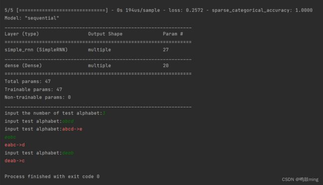
2.多个字母输入
输入4字母, 预测第5个字母
| X(输入) | Y(输出) |
|---|---|
| abcd | e |
| bcde | a |
| cdea | b |
| deab | c |
| eabc | d |

import numpy as np
import tensorflow as tf
from tensorflow.keras.layers import Dense, SimpleRNN
import matplotlib.pyplot as plt
import os

input_word = "abcde"
w_to_id = {'a': 0, 'b': 1, 'c': 2, 'd': 3, 'e': 4}  # 单词映射到数值id的词典
id_to_onehot = {0: [1., 0., 0., 0., 0.], 1: [0., 1., 0., 0., 0.], 2: [0., 0., 1., 0., 0.], 3: [0., 0., 0., 1., 0.],
                4: [0., 0., 0., 0., 1.]}  # id编码为one-hot

x_train = [
    [id_to_onehot[w_to_id['a']], id_to_onehot[w_to_id['b']], id_to_onehot[w_to_id['c']], id_to_onehot[w_to_id['d']]],
    [id_to_onehot[w_to_id['b']], id_to_onehot[w_to_id['c']], id_to_onehot[w_to_id['d']], id_to_onehot[w_to_id['e']]],
    [id_to_onehot[w_to_id['c']], id_to_onehot[w_to_id['d']], id_to_onehot[w_to_id['e']], id_to_onehot[w_to_id['a']]],
    [id_to_onehot[w_to_id['d']], id_to_onehot[w_to_id['e']], id_to_onehot[w_to_id['a']], id_to_onehot[w_to_id['b']]],
    [id_to_onehot[w_to_id['e']], id_to_onehot[w_to_id['a']], id_to_onehot[w_to_id['b']], id_to_onehot[w_to_id['c']]],
]
y_train = [w_to_id['e'], w_to_id['a'], w_to_id['b'], w_to_id['c'], w_to_id['d']]

np.random.seed(7)
np.random.shuffle(x_train)
np.random.seed(7)
np.random.shuffle(y_train)
tf.random.set_seed(7)

# 使x_train符合SimpleRNN输入要求:[送入样本数, 循环核时间展开步数, 每个时间步输入特征个数]。
# 此处整个数据集送入,送入样本数为len(x_train);输入4个字母出结果,循环核时间展开步数为4; 表示为独热码有5个输入特征,每个时间步输入特征个数为5
x_train = np.reshape(x_train, (len(x_train), 4, 5))
y_train = np.array(y_train)

model = tf.keras.Sequential([
    SimpleRNN(3),
    Dense(5, activation='softmax')
])

model.compile(optimizer=tf.keras.optimizers.Adam(0.01),
              loss=tf.keras.losses.SparseCategoricalCrossentropy(from_logits=False),
              metrics=['sparse_categorical_accuracy'])

# checkpoint_save_path = "./checkpoint/rnn_onehot_4pre1.ckpt"
#
# if os.path.exists(checkpoint_save_path + '.index'):
#     print('-------------load the model-----------------')
#     model.load_weights(checkpoint_save_path)
#
# cp_callback = tf.keras.callbacks.ModelCheckpoint(filepath=checkpoint_save_path,
#                                                  save_weights_only=True,
#                                                  save_best_only=True,
#                                                  monitor='loss')  # 由于fit没有给出测试集,不计算测试集准确率,根据loss,保存最优模型

# history = model.fit(x_train, y_train, batch_size=32, epochs=100, callbacks=[cp_callback])
history = model.fit(x_train, y_train, batch_size=32, epochs=100)
model.summary()

# print(model.trainable_variables)
# file = open('./weights.txt', 'w')  # 参数提取
# for v in model.trainable_variables:
#     file.write(str(v.name) + '\n')
#     file.write(str(v.shape) + '\n')
#     file.write(str(v.numpy()) + '\n')
# file.close()

###############################################    show   ###############################################

# 显示训练集和验证集的acc和loss曲线
acc = history.history['sparse_categorical_accuracy']
loss = history.history['loss']

plt.subplot(1, 2, 1)
plt.plot(acc, label='Training Accuracy')
plt.title('Training Accuracy')
plt.legend()

plt.subplot(1, 2, 2)
plt.plot(loss, label='Training Loss')
plt.title('Training Loss')
plt.legend()
plt.show()

############### predict #############

preNum = int(input("input the number of test alphabet:"))
for i in range(preNum):
    alphabet1 = input("input test alphabet:")
    alphabet = [id_to_onehot[w_to_id[a]] for a in alphabet1]
    # 使alphabet符合SimpleRNN输入要求:[送入样本数, 循环核时间展开步数, 每个时间步输入特征个数]。此处验证效果送入了1个样本,送入样本数为1;输入4个字母出结果,所以循环核时间展开步数为4; 表示为独热码有5个输入特征,每个时间步输入特征个数为5
    alphabet = np.reshape(alphabet, (1, 4, 5))
    result = model.predict([alphabet])
    pred = tf.argmax(result, axis=1)
    pred = int(pred)
    tf.print(alphabet1 + '->' + input_word[pred])
运行结果

3.Embedding 编码
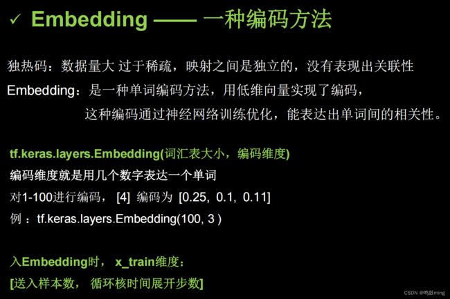
稍作修改


import numpy as np
import tensorflow as tf
from tensorflow.keras.layers import Dense, SimpleRNN, Embedding
import matplotlib.pyplot as plt
import os

input_word = "abcdefghijklmnopqrstuvwxyz"
w_to_id = {'a': 0, 'b': 1, 'c': 2, 'd': 3, 'e': 4,
           'f': 5, 'g': 6, 'h': 7, 'i': 8, 'j': 9,
           'k': 10, 'l': 11, 'm': 12, 'n': 13, 'o': 14,
           'p': 15, 'q': 16, 'r': 17, 's': 18, 't': 19,
           'u': 20, 'v': 21, 'w': 22, 'x': 23, 'y': 24, 'z': 25}  # 单词映射到数值id的词典

training_set_scaled = [0, 1, 2, 3, 4, 5, 6, 7, 8, 9, 10,
                       11, 12, 13, 14, 15, 16, 17, 18, 19, 20,
                       21, 22, 23, 24, 25]

x_train = []
y_train = []

for i in range(4, 26):
    x_train.append(training_set_scaled[i - 4:i])
    y_train.append(training_set_scaled[i])

np.random.seed(7)
np.random.shuffle(x_train)
np.random.seed(7)
np.random.shuffle(y_train)
tf.random.set_seed(7)

# 使x_train符合Embedding输入要求:[送入样本数, 循环核时间展开步数] ,
# 此处整个数据集送入所以送入,送入样本数为len(x_train);输入4个字母出结果,循环核时间展开步数为4。
x_train = np.reshape(x_train, (len(x_train), 4))
y_train = np.array(y_train)

model = tf.keras.Sequential([
    Embedding(26, 2),
    SimpleRNN(10),
    Dense(26, activation='softmax')
])

model.compile(optimizer=tf.keras.optimizers.Adam(0.01),
              loss=tf.keras.losses.SparseCategoricalCrossentropy(from_logits=False),
              metrics=['sparse_categorical_accuracy'])
#
# checkpoint_save_path = "./checkpoint/rnn_embedding_4pre1.ckpt"
#
# if os.path.exists(checkpoint_save_path + '.index'):
#     print('-------------load the model-----------------')
#     model.load_weights(checkpoint_save_path)
#
# cp_callback = tf.keras.callbacks.ModelCheckpoint(filepath=checkpoint_save_path,
#                                                  save_weights_only=True,
#                                                  save_best_only=True,
#                                                  monitor='loss')  # 由于fit没有给出测试集,不计算测试集准确率,根据loss,保存最优模型

# history = model.fit(x_train, y_train, batch_size=32, epochs=100, callbacks=[cp_callback])
history = model.fit(x_train, y_train, batch_size=32, epochs=100)
model.summary()

# file = open('./weights.txt', 'w')  # 参数提取
# for v in model.trainable_variables:
#     file.write(str(v.name) + '\n')
#     file.write(str(v.shape) + '\n')
#     file.write(str(v.numpy()) + '\n')
# file.close()

###############################################    show   ###############################################

# 显示训练集和验证集的acc和loss曲线
acc = history.history['sparse_categorical_accuracy']
loss = history.history['loss']

plt.subplot(1, 2, 1)
plt.plot(acc, label='Training Accuracy')
plt.title('Training Accuracy')
plt.legend()

plt.subplot(1, 2, 2)
plt.plot(loss, label='Training Loss')
plt.title('Training Loss')
plt.legend()
plt.show()

################# predict ##################

preNum = int(input("input the number of test alphabet:"))
for i in range(preNum):
    alphabet1 = input("input test alphabet:")
    alphabet = [w_to_id[a] for a in alphabet1]
    # 使alphabet符合Embedding输入要求:[送入样本数, 时间展开步数]。
    # 此处验证效果送入了1个样本,送入样本数为1;输入4个字母出结果,循环核时间展开步数为4。
    alphabet = np.reshape(alphabet, (1, 4))
    result = model.predict([alphabet])
    pred = tf.argmax(result, axis=1)
    pred = int(pred)
    tf.print(alphabet1 + '->' + input_word[pred])
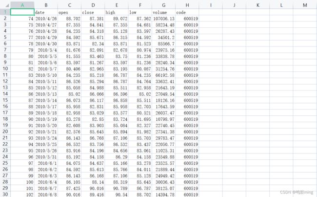
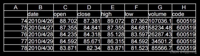
3.预测股票
1.数据源
数据下载:https://download.csdn.net/download/qq_41865229/85244420
2.代码
import numpy as np
import tensorflow as tf
from tensorflow.keras.layers import Dropout, Dense, SimpleRNN
import matplotlib.pyplot as plt
import os
import pandas as pd
from sklearn.preprocessing import MinMaxScaler
from sklearn.metrics import mean_squared_error, mean_absolute_error
import math
maotai = pd.read_csv('./SH600519.csv') # 读取股票文件
training_set = maotai.iloc[0:2426 - 300, 2:3].values # 前(2426-300=2126)天的开盘价作为训练集,表格从0开始计数,2:3 是提取[2:3)列,前闭后开,故提取出C列开盘价
test_set = maotai.iloc[2426 - 300:, 2:3].values # 后300天的开盘价作为测试集
# 归一化
sc = MinMaxScaler(feature_range=(0, 1)) # 定义归一化:归一化到(0,1)之间
training_set_scaled = sc.fit_transform(training_set) # 求得训练集的最大值,最小值这些训练集固有的属性,并在训练集上进行归一化
test_set = sc.transform(test_set) # 利用训练集的属性对测试集进行归一化
x_train = []
y_train = []
x_test = []
y_test = []
# 测试集:csv表格中前2426-300=2126天数据
# 利用for循环,遍历整个训练集,提取训练集中连续60天的开盘价作为输入特征x_train,第61天的数据作为标签,for循环共构建2426-300-60=2066组数据。
for i in range(60, len(training_set_scaled)):
x_train.append(training_set_scaled[i - 60:i, 0])
y_train.append(training_set_scaled[i, 0])
# 对训练集进行打乱
np.random.seed(7)
np.random.shuffle(x_train)
np.random.seed(7)
np.random.shuffle(y_train)
tf.random.set_seed(7)
# 将训练集由list格式变为array格式
x_train, y_train = np.array(x_train), np.array(y_train)
# 使x_train符合RNN输入要求:[送入样本数, 循环核时间展开步数, 每个时间步输入特征个数]。
# 此处整个数据集送入,送入样本数为x_train.shape[0]即2066组数据;输入60个开盘价,预测出第61天的开盘价,循环核时间展开步数为60; 每个时间步送入的特征是某一天的开盘价,只有1个数据,故每个时间步输入特征个数为1
x_train = np.reshape(x_train, (x_train.shape[0], 60, 1))
# 测试集:csv表格中后300天数据
# 利用for循环,遍历整个测试集,提取测试集中连续60天的开盘价作为输入特征x_train,第61天的数据作为标签,for循环共构建300-60=240组数据。
for i in range(60, len(test_set)):
x_test.append(test_set[i - 60:i, 0])
y_test.append(test_set[i, 0])
# 测试集变array并reshape为符合RNN输入要求:[送入样本数, 循环核时间展开步数, 每个时间步输入特征个数]
x_test, y_test = np.array(x_test), np.array(y_test)
x_test = np.reshape(x_test, (x_test.shape[0], 60, 1))
model = tf.keras.Sequential([
SimpleRNN(80, return_sequences=True),
Dropout(0.2),
SimpleRNN(100),
Dropout(0.2),
Dense(1)
])
model.compile(optimizer=tf.keras.optimizers.Adam(0.001),
loss='mean_squared_error') # 损失函数用均方误差
# 该应用只观测loss数值,不观测准确率,所以删去metrics选项,一会在每个epoch迭代显示时只显示loss值
checkpoint_save_path = "./rnn/checkpoint/rnn_stock.ckpt"
if os.path.exists(checkpoint_save_path + '.index'):
print('-------------load the model-----------------')
model.load_weights(checkpoint_save_path)
cp_callback = tf.keras.callbacks.ModelCheckpoint(filepath=checkpoint_save_path,
save_weights_only=True,
save_best_only=True,
monitor='val_loss')
history = model.fit(x_train, y_train, batch_size=64, epochs=50, validation_data=(x_test, y_test), validation_freq=1,
callbacks=[cp_callback])
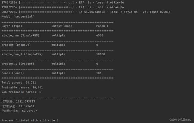
model.summary()
file = open('./rnn/weights.txt', 'w') # 参数提取
for v in model.trainable_variables:
file.write(str(v.name) + '\n')
file.write(str(v.shape) + '\n')
file.write(str(v.numpy()) + '\n')
file.close()
loss = history.history['loss']
val_loss = history.history['val_loss']
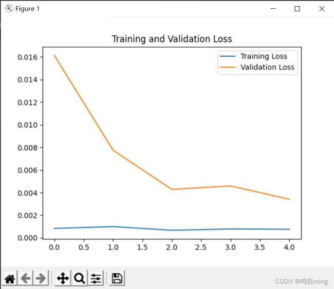
plt.plot(loss, label='Training Loss')
plt.plot(val_loss, label='Validation Loss')
plt.title('Training and Validation Loss')
plt.legend()
plt.show()
################## predict ######################
# 测试集输入模型进行预测
predicted_stock_price = model.predict(x_test)
# 对预测数据还原---从(0,1)反归一化到原始范围
predicted_stock_price = sc.inverse_transform(predicted_stock_price)
# 对真实数据还原---从(0,1)反归一化到原始范围
real_stock_price = sc.inverse_transform(test_set[60:])
# 画出真实数据和预测数据的对比曲线
plt.plot(real_stock_price, color='red', label='MaoTai Stock Price')
plt.plot(predicted_stock_price, color='blue', label='Predicted MaoTai Stock Price')
plt.title('MaoTai Stock Price Prediction')
plt.xlabel('Time')
plt.ylabel('MaoTai Stock Price')
plt.legend()
plt.show()
##########evaluate##############
# calculate MSE 均方误差 ---> E[(预测值-真实值)^2] (预测值减真实值求平方后求均值)
mse = mean_squared_error(predicted_stock_price, real_stock_price)
# calculate RMSE 均方根误差--->sqrt[MSE] (对均方误差开方)
rmse = math.sqrt(mean_squared_error(predicted_stock_price, real_stock_price))
# calculate MAE 平均绝对误差----->E[|预测值-真实值|](预测值减真实值求绝对值后求均值)
mae = mean_absolute_error(predicted_stock_price, real_stock_price)
print('均方误差: %.6f' % mse)
print('均方根误差: %.6f' % rmse)
print('平均绝对误差: %.6f' % mae)
运行结果