天猫复购预测

课设人员

张芳

目录

课设人员

课题主要内容

思路：

数据描述

​编辑 处理过程

 数据探索

数据初步可视化

---

课题主要内容

需要根据天猫复购预测中提供的数据，来预测新买家在未来六个月内再次在同一个商家购买商品的概率。

思路：

用LR的预测结果作为baseline;然后分别用XGBoost，LightGBM，CatBoost，DIN，NGBoost，K折xgb+lgb+catb模型融合进行训练并预测，与baseline效果对比，发现lgb和xgb速度和效果都不错，单模型中catboost效果最好，应该是分类特征比较多的故缘;然后DIN效果并不理想，且运行时间较长，模型泛用性较差;而3种boost模型融合效果有小幅度提升，但是运算时间比单一方法长很多。

数据描述

文件

字段描述：

 

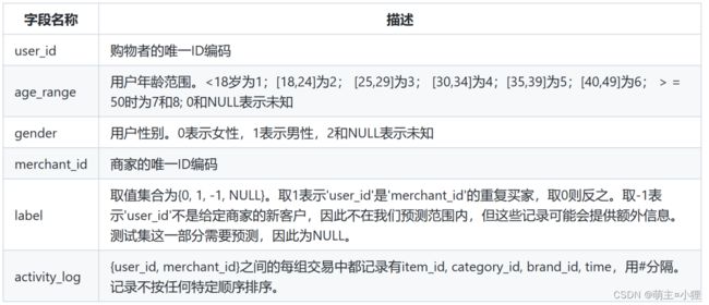
用户行为：

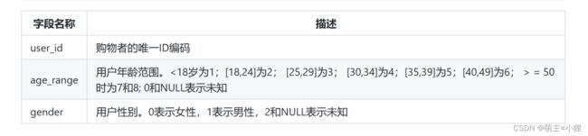
 用户画像：

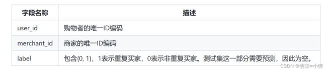
 训练数据和测试数据：

结果保存：

 处理过程

 数据探索

导入相关的数据包：

import numpy as np
import pandas as pd
import matplotlib.pyplot as plt
plt.rcParams["font.sans-serif"] = "SimHei" #解决中文乱码问题
import seaborn as sns
import random
from sklearn.model_selection import train_test_split
from sklearn.linear_model import LogisticRegression
from sklearn.preprocessing import LabelEncoder
from sklearn.metrics import accuracy_score
from sklearn import model_selection
from sklearn.neighbors import KNeighborsRegressor

读取数据：

df_train = pd.read_csv(r'E:\python  xue\课设\suju\data_format1\train_format1.csv')
df_test = pd.read_csv(r'E:\python  xue\课设\suju\data_format1\test_format1.csv')
user_info = pd.read_csv(r'E:\python  xue\课设\suju\data_format1\user_info_format1.csv')
user_log = pd.read_csv(r'E:\python  xue\课设\suju\data_format1\user_log_format1.csv')

读取数据大小：

利用numpy中的shape函数来读取矩阵的长度，得到一个tuple格式的数据，之后也可以使用
shape[ ] 来获取其中需要的收据

print(df_test.shape,df_train.shape)
print(user_info.shape,user_log.shape)

结果：(261477, 3) (260864, 3)
(424170, 3) (54925330, 7)

缺失值查看及预处理：

显示给出样本数据的相关信息概览 ：行数，列数，列索引，列非空值个数，列类型，内存占用

用户信息数据

        数据集中共有2个float64类型和1个int64类型的数据
        数据大小9.7MB
        数据集共有424170条数据

用户行为数据

        数据集中共有6个int64类型和1个float64类型的数据
        数据大小2.9GB
        数据集共有54925330条数据

用户购买训练数据

        数据均为int64类型
        数据大小6MB
        数据集共有260864条数据

user_info.head(10)

user_id	age_range	gender
0	376517	6.0	1.0
1	234512	5.0	0.0
2	344532	5.0	0.0
3	186135	5.0	0.0
4	30230	5.0	0.0
5	272389	6.0	1.0
6	281071	4.0	0.0
7	139859	7.0	0.0
8	198411	5.0	1.0
9	67037	4.0	1.0

user_info['age_range'].replace(0.0,np.nan,inplace=True)
user_info['gender'].replace(2.0,np.nan,inplace=True)
user_info.info()

RangeIndex: 424170 entries, 0 to 424169
Data columns (total 3 columns):
 #   Column     Non-Null Count   Dtype  
---  ------     --------------   -----  
 0   user_id    424170 non-null  int64  
 1   age_range  329039 non-null  float64
 2   gender     407308 non-null  float64
dtypes: float64(2), int64(1)
memory usage: 9.7 MB

user_info['age_range'].replace(np.nan,-1,inplace=True)
user_info['gender'].replace(np.nan,-1,inplace=True)
fig = plt.figure(figsize = (10, 6))
x = np.array(["NULL","<18","18-24","25-29","30-34","35-39","40-49",">=50"])
#<18岁为1；[18,24]为2； [25,29]为3； [30,34]为4；[35,39]为5；[40,49]为6； > = 50时为7和8
y = np.array([user_info[user_info['age_range'] == -1]['age_range'].count(),
             user_info[user_info['age_range'] == 1]['age_range'].count(),
             user_info[user_info['age_range'] == 2]['age_range'].count(),
             user_info[user_info['age_range'] == 3]['age_range'].count(),
             user_info[user_info['age_range'] == 4]['age_range'].count(),
             user_info[user_info['age_range'] == 5]['age_range'].count(),
             user_info[user_info['age_range'] == 6]['age_range'].count(),
             user_info[user_info['age_range'] == 7]['age_range'].count() + user_info[user_info['age_range'] == 8]['age_range'].count()])
plt.bar(x,y,label='人数')
plt.legend()
plt.title('用户年龄分布')

 

sns.countplot(x = 'age_range', order = [-1,1,2,3,4,5,6,7,8], data = user_info)
plt.title('用户年龄分布')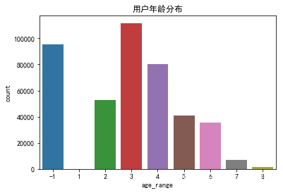

sns.countplot(x='gender',order = [-1,0,1],data = user_info)
plt.title('用户性别分布')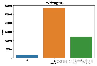

 

sns.countplot(x = 'age_range', order = [-1,1,2,3,4,5,6,7,8],hue= 'gender',data = user_info)
plt.title('用户性别年龄分布')

分析总结:

年龄的缺失值较多，性别的缺失值较少，用户年龄主要分布到18~34岁，主要群体为女性。 

数据查看及统计：

user_log.head()

	user_id	item_id	cat_id	seller_id	brand_id	time_stamp	action_type
0	328862	323294	833	2882	2661.0	829	0
1	328862	844400	1271	2882	2661.0	829	0
2	328862	575153	1271	2882	2661.0	829	0
3	328862	996875	1271	2882	2661.0	829	0
4	328862	1086186	1271	1253	1049.0	829	0

user_log.isnull().sum(axis=0)

user_id            0
item_id            0
cat_id             0
seller_id          0
brand_id       91015
time_stamp         0
action_type        0
dtype: int64

user_log.isnull().sum(axis=0)

user_id            0
item_id            0
cat_id             0
seller_id          0
brand_id       91015
time_stamp         0
action_type        0
dtype: int64

user_log.info()#对于用户日志里的商品品牌的缺失也做了删除处理

RangeIndex: 54925330 entries, 0 to 54925329
Data columns (total 7 columns):
 #   Column       Dtype  
---  ------       -----  
 0   user_id      int64  
 1   item_id      int64  
 2   cat_id       int64  
 3   seller_id    int64  
 4   brand_id     float64
 5   time_stamp   int64  
 6   action_type  int64  
dtypes: float64(1), int64(6)
memory usage: 2.9 GB

数据初步可视化

• user_log前面几行全是编码，购物者的唯一ID编码，商品的唯一编码，商品所属品类的唯一编码，商家的唯一ID编码，商品品牌的唯一编码
• 后面是购买时间，与活动日志记录

df_train.head(10)

	user_id	merchant_id	label
0	34176	3906	0
1	34176	121	0
2	34176	4356	1
3	34176	2217	0
4	230784	4818	0
5	362112	2618	0
6	34944	2051	0
7	231552	3828	1
8	231552	2124	0
9	232320	1168	0

df_train.info()

RangeIndex: 260864 entries, 0 to 260863
Data columns (total 3 columns):
 #   Column       Non-Null Count   Dtype
---  ------       --------------   -----
 0   user_id      260864 non-null  int64
 1   merchant_id  260864 non-null  int64
 2   label        260864 non-null  int64
dtypes: int64(3)
memory usage: 6.0 MB

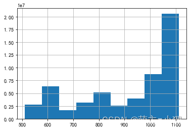
user_log['time_stamp'].hist(bins = 9)

 618和双十一购物量较多

sns.countplot(x = 'action_type', order = [0,1,2,3],data = user_log)

 绝大多数都是单击，加入购物车的动作很少，比购买和收藏的动作还要少

 特征工程：

df_train[df_train['label'] == 1]

	user_id	merchant_id	label
2	34176	4356	1
7	231552	3828	1
53	306816	1489	1
57	176256	3323	1
59	307584	1340	1
...	...	...	...
260747	208511	2592	1
260793	87935	1964	1
260794	87935	3734	1
260799	350591	4394	1
260842	422783	2026	1

建立特征
需要根据user_id，和merchant_id（seller_id）,从用户画像表以及用户日志表中提取特征，填写到df_train这个数据框中，从而训练评估模型
需要建立的特征如下：
用户的年龄(age_range)
用户的性别(gender)
某用户在该商家日志的总条数(total_logs)
用户浏览的商品的数目，就是浏览了多少个商品(unique_item_ids)
浏览的商品的种类的数目，就是浏览了多少种商品(categories)
用户浏览的天数(browse_days)
用户单击的次数(one_clicks)
用户添加购物车的次数(shopping_carts)
用户购买的次数(purchase_times)
用户收藏的次数(favourite_times)

df_train.head()
user_info.head()
user_log.head()
df_train = pd.merge(df_train,user_info,on="user_id",how="left")
df_train.head()