Classification techniques are an important part of machine learning and data mining applications. Approx 70% of problems in Data Science are classification problems. There are lots of classification problems are available but the logistics regression is a very common and useful regression method for solving a binary classification problem. Another category of classification is Multinomial classification, which handles the problems where multiple classes are present in the target variable. For example, the IRIS dataset various famous examples of multiclass classification. Other examples are classifying article/blog/document categories.
分类技术是机器学习和数据挖掘应用程序的重要组成部分。 数据科学中大约70%的问题是分类问题。 存在许多分类问题,但是物流回归是解决二元分类问题的非常普遍且有用的回归方法。 分类的另一种类别是多项式分类,它可以处理目标变量中存在多个类别的问题。 例如,IRIS数据集各种著名的多类分类示例。 其他示例是对文章/博客/文档类别进行分类。
Logistic Regression can be used for various classification problems such as spam detection, Diabetes prediction, if a given customer will purchase a particular product or will churn to another competitor, the user will click on a given advertisement link or not and many more examples are in the bucket.
Logistic回归可用于各种分类问题,例如垃圾邮件检测,糖尿病预测,如果给定的客户将购买特定产品或将其吸引到其他竞争对手,则用户是否会点击给定的广告链接,并且还有更多示例桶。
Logistic Regression is one of the most simple and commonly used Machine Learning algorithms for two-class classification. It is easy to implement and can be used as the baseline for any binary classification problem. Its basic fundamental concepts are also very helpful in deep learning. Logistic regression describes and estimates the relationship between one dependent binary variable and independent variables.
Logistic回归是用于两类分类的最简单,最常用的机器学习算法之一。 它易于实现,并且可以用作任何二进制分类问题的基准。 它的基本概念对深度学习也很有帮助。 Logistic回归描述和估计一个因变量和自变量之间的关系。
In this tutorial, you will learn the following things in Logistic Regression:
在本教程中,您将在Logistic回归中学习以下内容:
- Introduction to Logistic Regression Logistic回归简介
- Linear Regression Vs. Logistic Regression 线性回归与 逻辑回归
- Maximum Likelihood Estimation Vs. Ordinary Least Square Method 最大似然估计与 普通最小二乘法
- How do Logistic Regression works? Logistic回归如何工作?
- Model building in Scikit-learn Scikit-learn中的模型构建
- Model Evaluation using Confusion Matrix and ROC Curve. 使用混淆矩阵和ROC曲线进行模型评估。
- Advantages and Disadvantages of Logistic Regression Logistic回归的优缺点
逻辑回归 (Logistic Regression)
Logistic regression is a statistical method for predicting binary classes. The outcome or target variable is dichotomous in nature, dichotomous means there are only two possible classes. for example, it can be used for cancer detection problems. It computes the probability of an event occurrence.
Logistic回归是用于预测二进制类别的统计方法。 结果或目标变量本质上是二分的,二分意味着只有两种可能的类别。 例如,它可以用于癌症检测问题。 它计算事件发生的概率。
It is a special case of linear regression where the target variable is categorical in nature. It uses a log of odds as the dependent variable. Logistic Regression predicts the probability of occurrence of a binary event using a logit function.
这是线性回归的一种特殊情况,其中目标变量本质上是分类的。 它使用几率对数作为因变量。 Logistic回归使用logit函数预测二进制事件的发生概率。
Linear Regression Equation:
线性回归方程:
Where, y is the dependent variable and x1, x2 … and Xn are explanatory variables.
其中,y是因变量,x1,x2…和Xn是解释变量。
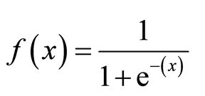
Sigmoid Function:
乙状结肠功能:
Apply Sigmoid function on linear regression:
将Sigmoid函数应用于线性回归:
Properties of Logistic Regression:
Logistic回归的属性:
- The dependent variable in logistic regression follows Bernoulli Distribution. 逻辑回归中的因变量遵循伯努利分布。
- Estimation is done through maximum likelihood. 估计是通过最大似然来完成的。
- No R Square, Model fitness is calculated through Concordance, KS-Statistics. 没有R平方,模型适用性通过Concordance,KS-Statistics计算。
线性回归与 逻辑回归 (Linear Regression Vs. Logistic Regression)
Linear regression gives you a continuous output but logistic regression gives a continuous output. An example of a continuous output is house price and stock price. An example of the discrete output is predicting whether a patient has cancer or not, predicting whether the customer will churn. Linear regression is estimated using Ordinary Least Squares (OLS) while logistic regression is estimated using the Maximum Likelihood Estimation (MLE) approach.
线性回归可提供连续输出,而逻辑回归可提供连续输出。 连续输出的一个例子是房屋价格和股票价格。 离散输出的一个例子是预测患者是否患有癌症,预测客户是否会流失。 使用普通最小二乘(OLS)估计线性回归,而使用最大似然估计(MLE)方法估计逻辑回归。
最大似然估计与 最小二乘法 (Maximum Likelihood Estimation Vs. Least Square Method)
The MLE is a “likelihood” maximization method, while OLS is a distance-minimizing approximation method. Maximizing the likelihood function determines the parameters that are most likely to produce the observed data. From a statistical point of view, MLE sets the mean and variance as parameters in determining the specific parametric values for a given model. This set of parameters can be used for predicting the data needed in a normal distribution.
MLE是一种“可能性”最大化方法,而OLS是一种距离最小化近似方法。 最大化似然函数可确定最有可能产生观测数据的参数。 从统计角度来看,MLE将平均值和方差设置为确定给定模型的特定参数值的参数。 这组参数可用于预测正态分布中所需的数据。
Ordinary Least squares estimates are computed by fitting a regression line on given data points that has the minimum sum of the squared deviations (least square error). Both are used to estimate the parameters of a linear regression model. MLE assumes a joint probability mass function, while OLS doesn’t require any stochastic assumptions for minimizing distance.
普通最小二乘估计值是通过在给定的数据点上拟合回归线而得出的,该数据点具有平方差的最小和(最小二乘误差)。 两者都用于估计线性回归模型的参数。 MLE假设一个联合概率质量函数,而OLS不需要任何随机假设来最小化距离。
乙状结肠功能 (Sigmoid Function)
The sigmoid function also called the logistic function gives an ‘S’ shaped curve that can take any real-valued number and map it into a value between 0 and 1. If the curve goes to positive infinity, y predicted will become 1 and If the curve goes to negative infinity, y predicted will become 0. If the output of sigmoid function more than 0.5, we can classify the outcome as 1 or YES and if it is less than 0.5, we can classify it as 0 or NO. The outputcannotFor example: If the output is 0.75, we can say in terms of probability as: There is a 75 percent chance that the patient will suffer from cancer.
S形函数也称为对数函数,它给出的曲线为S形,可以采用任何实数值并将其映射为0到1之间的值。如果曲线变为正无穷大,则y的预测值将变为1,而如果曲线变为负无穷大,则y预测将变为0。如果S型函数的输出大于0.5,则可以将结果分类为1或是,如果结果小于0.5,则可以将其分类为0或NO。 输出不能为例如:如果输出为0.75,就概率而言,我们可以这样说:患者有75%的机会患上癌症。
Logistic回归的类型 (Types of Logistic Regression)
Types of Logistic Regression:
Logistic回归的类型:
- Binary Logistic Regression: The target variable has only two possible outcomes such as Spam or Not Spam, Cancer, or No Cancer. 二进制Logistic回归:目标变量只有两个可能的结果,例如垃圾邮件或非垃圾邮件,癌症或没有癌症。
- Multinomial Logistic Regression: The target variable has three or more nominal categories such as predicting the type of Wine. 多项逻辑回归:目标变量具有三个或更多名义类别,例如预测酒的类型。
- Ordinal Logistic Regression: the target variable has three or more ordinal categories such as restaurant or product rating from 1 to 5. 序数逻辑回归:目标变量具有三个或更多序数类别,例如餐厅或产品等级从1到5。
Scikit-learn中的模型构建 (Model building in Scikit-learn)
Let’s build a diabetes prediction model.
让我们建立一个糖尿病预测模型。
Here, you are going to predict diabetes using a Logistic Regression Classifier.
在这里,您将使用Logistic回归分类器预测糖尿病。
Let’s first load the required Pima Indian Diabetes dataset using pandas’ read CSV function. You can download data from the following link:
我们首先使用熊猫的read CSV函数加载所需的Pima印度糖尿病数据集。 您可以从以下链接下载数据:
加载数据中 (Loading Data)
#import pandasimport pandas as pdcol_names = ['pregnant', 'glucose', 'bp', 'skin', 'insulin', 'bmi', 'pedigree', 'age', 'label']# load datasetpima = pd.read_csv("pima-indians-diabetes.csv", header=None, names=col_names)pima.head()选择特征 (Selecting Feature)
Here, you need to divide given columns into two types of variables dependent(or target variable) and independent variable(or feature variables).
在这里,您需要将给定的列分为因变量(目标变量)和自变量(或特征变量)两种类型。
#split dataset in features and target variablefeature_cols = ['pregnant', 'insulin', 'bmi', 'age','glucose','bp','pedigree']X = pima[feature_cols] # Featuresy = pima.label # Target variable分割数据 (Splitting Data)
To understand model performance, dividing the dataset into a training set and a test set is a good strategy.
为了了解模型的性能,将数据集分为训练集和测试集是一个很好的策略。
Let’s split dataset by using function train_test_split(). you need to pass basically 3 parameters features, target, and test_set size. Additionally, you can use random_state to select records randomly.
让我们使用函数train_test_split()拆分数据集。 您基本上需要通过3个参数功能,目标和test_set大小。 此外,您可以使用random_state随机选择记录。
# split X and y into training and testing setsfrom sklearn.cross_validation import train_test_splitX_train,X_test,y_train,y_test=train_test_split(X,y,test_size=0.25,random_state=0)Here, Dataset is broken into two parts in the ratio of 75:25. It means 75% of data will be used for model training and 25% for model testing.
在这里,数据集按75:25的比例分为两部分。 这意味着75%的数据将用于模型训练,而25%的数据将用于模型测试。
模型开发与预测 (Model Development and Prediction)
First, import the Logistic Regression module and create a Logistic Regression classifier object using the LogisticRegression() function.
首先,导入Logistic回归模块,并使用LogisticRegression()函数创建一个Logistic回归分类器对象。
Then, fit your model on the train set using fit() and perform prediction on the test set using predict().
然后,使用fit()将模型拟合到训练集上,并使用predict()对测试集执行预测。
# import the classfrom sklearn.linear_model import LogisticRegression# instantiate the model (using the default parameters)logreg = LogisticRegression()# fit the model with datalogreg.fit(X_train,y_train)
# predict y_pred=logreg.predict(X_test)使用混淆矩阵的模型评估 (Model Evaluation using Confusion Matrix)
A confusion matrix is a table that is used to evaluate the performance of a classification model. You can also visualize the performance of an algorithm. The fundamental of a confusion matrix is the number of correct and incorrect predictions are summed up class-wise.
混淆矩阵是用于评估分类模型的性能的表。 您还可以可视化算法的性能。 混淆矩阵的基本原理是按类别汇总正确和错误预测的数量。
In [9]:
在[9]中:
# import the metrics classfrom sklearn import metricscnf_matrix = metrics.confusion_matrix(y_test, y_pred)cnf_matrix
Output:array([[119,  11],
       [ 26,  36]])
Here, you can see the confusion matrix in the form of an array object. The dimension of this matrix is 2*2 because this model is a binary classification. you have two classes 0 and 1. Diagonal values represent accurate predictions, while non-diagonal elements are inaccurate predictions. In the output, 119 and 36 are actual predictions and 26 and 11 are inaccurate predictions.
在这里,您可以看到数组对象形式的混淆矩阵。 该矩阵的维数为2 * 2,因为该模型是二进制分类。 您有两个类别0和1。对角线值表示准确的预测,而非对角线元素则表示不正确的预测。 在输出中,119和36是实际预测,而26和11是不准确的预测。
使用热图可视化混淆矩阵 (Visualizing Confusion Matrix using Heatmap)
Let’s visualize the results of the model in the form of a confusion matrix using matplotlib and seaborn.
让我们使用matplotlib和seaborn以混淆矩阵的形式可视化模型的结果。
Here, you will visualize the confusion matrix using Heatmap.
在这里,您将使用Heatmap可视化混淆矩阵。
# import required modulesimport numpy as npimport matplotlib.pyplot as pltimport seaborn as sns%matplotlib inline
class_names=[0,1] # name  of classesfig, ax = plt.subplots()tick_marks = np.arange(len(class_names))plt.xticks(tick_marks, class_names)plt.yticks(tick_marks, class_names)# create heatmapsns.heatmap(pd.DataFrame(cnf_matrix), annot=True, cmap="YlGnBu" ,fmt='g')ax.xaxis.set_label_position("top")plt.tight_layout()plt.title('Confusion matrix', y=1.1)plt.ylabel('Actual label')plt.xlabel('Predicted label')
混淆矩阵评估指标 (Confusion Matrix Evaluation Metrics)
Let’s evaluate the model using model evaluation metrics such as accuracy, precision, and recall.
让我们使用模型评估指标(例如准确性,准确性和召回率)评估模型。
print("Accuracy:",metrics.accuracy_score(y_test, y_pred))print("Precision:",metrics.precision_score(y_test, y_pred))print("Recall:",metrics.recall_score(y_test, y_pred))Output:Accuracy: 0.8072916666666666
Precision: 0.7659574468085106
Recall: 0.5806451612903226
Well, you got a classification rate of 80%, considered as good accuracy.
好吧,您的分类率为80%,被认为是不错的准确性。
Precision: Precision is about being precise i.e. How precise your model is. In other words, you can say, when a model makes a prediction, how often it is correct. In your prediction case, when your Logistic Regression model predicted patients are going to suffer from diabetes, that patients actually have 76% time.
精度:精度是指精度,即模型的精度。 换句话说,您可以说,当模型做出预测时,它正确的频率是多少。 在您的预测案例中,当您的Logistic回归模型预测患者将要患糖尿病时,该患者实际上有76%的时间。
Recall: If there are patients who actually have diabetes in the test set and your Logistic Regression model is able to identify it 58% of the time.
回想一下:如果测试集中确实有糖尿病患者,并且您的Logistic回归模型能够在58%的时间内识别出糖尿病。
ROC曲线 (ROC Curve)
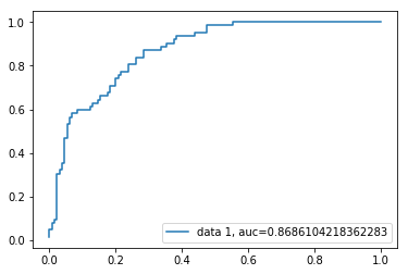
The Receiver Operating Characteristic(ROC) curve is a plot of the true positive rate against the false-positive rate. It shows the tradeoff between sensitivity and specificity.
接收器工作特性(ROC)曲线是真实的阳性率与假阳性率的关系图。 它显示了敏感性和特异性之间的权衡。
y_pred_proba = logreg.predict_proba(X_test)[::,1]fpr, tpr, _ = metrics.roc_curve(y_test, y_pred_proba)auc = metrics.roc_auc_score(y_test, y_pred_proba)plt.plot(fpr,tpr,label="data 1, auc="+str(auc))plt.legend(loc=4)plt.show()The AUC score for the case is 0.86. AUC score 1 represents a perfect classifier and 0.5 represents a worthless classifier.
该案件的AUC分数是0.86。 AUC得分1代表完美的分类器,而0.5代表毫无价值的分类器。
优点 (Advantages)
Because of its simple and efficient nature, doesn’t require high computation power, easy to implement, easily interpretable, used widely by data analyst and scientist. Also doesn’t require scaling of features. Logistic regression provides a probability score for observations.
由于其简单高效的性质,因此不需要高计算能力,易于实现,易于解释,并且被数据分析师和科学家广泛使用。 也不需要缩放功能。 Logistic回归为观察提供了概率分数。
缺点 (Disadvantages)
Logistic regression is not able to handle a large number of categorical features/variables. It is vulnerable to overfitting. Also, can’t solve the non-linear problem with the logistic regression that is why it requires a transformation of non-linear features. logistic regression will not perform well with independent variables that are not correlated to the target variable and very similar or correlated to each other.
Logistic回归无法处理大量分类特征/变量。 它很容易过拟合。 此外,无法通过逻辑回归来解决非线性问题,这就是为什么它需要转换非线性特征的原因。 如果逻辑变量与目标变量不相关,非常相似或彼此相关,则逻辑回归将无法很好地执行。
结论 (Conclusion)
In this tutorial, you covered a lot of details about Logistic Regression. you have learned what is the logistic regression, how to build respective models, how to visualize results, and some of the theoretical background information. Also, you covered some basic concepts such as the sigmoid function, maximum likelihood, confusion matrix, ROC curve.
在本教程中,您涵盖了有关Logistic回归的许多详细信息。 您已经了解了什么是逻辑回归,如何构建各自的模型,如何可视化结果以及一些理论背景信息。 此外,您还介绍了一些基本概念,例如S型函数,最大似然,混淆矩阵,ROC曲线。
Hopefully, you can now utilize the Logistic Regression technique to analyze your own datasets. Thanks for reading this tutorial!
希望您现在可以使用Logistic回归技术来分析自己的数据集。 感谢您阅读本教程!
For more such tutorials, projects, and courses visit DataCamp
有关更多此类教程,项目和课程的信息,请访问DataCamp
Originally published at https://www.datacamp.com/community/tutorials/understanding-logistic-regression-python
最初发布在https://www.datacamp.com/community/tutorials/understanding-logistic-regression-python
Reach out to me on Linkedin: https://www.linkedin.com/in/avinash-navlani/
在Linkedin上与我联系: https : //www.linkedin.com/in/avinash-navlani/
翻译自: https://medium.com/python-in-plain-english/understanding-logistic-regression-and-building-model-in-python-1752a7e562a8


