爆肝总结:神经网络大杂烩
文章目录
-
-
- purpose:
- 来龙去脉
- LeNet5
- Alexnet
- VGG
- Google Inception
- ResNet
- DenseNet
-
purpose:
论文里面经常会有对比实验,经常会用到一些较经典的网络。例如Alexnet网络是从Imagenet大赛中脱颖而出的模型,但是其原始的输入大小与输出大小可能与我们的任务并不相符。这种情况我们怎么使用经典的网络结构来做对比实验呢?
看过了一些论文复现的代码,大多数作者是这样处理的:
- 尽量保留经典模型的网络结构。如果任务不同,该改的还是要改。也就是说,他们复现的经典网络结构与其真实的本貌并不完全相同
在此,将常用网络模型的来源,实现以及其结构图总结起来,以便日后翻阅。如下内容实现的神经网络类,均可以运行。举例如下:
batch_size = 10
x = torch.rand(3,224,224)
x = x.expand(batch_size,*x.size())
model = DenseNet121(init_channel=60)
out = model(x)
print (out.shape)
Tips:
- 如下网络模型代码不一定完全符合其本貌。但会最大限度的使其相似。
来龙去脉
(1)理论萌芽阶段。1962年Hubel以及Wiesel通过生物学研究表明,从视网膜传递脑中的视觉信息是通过多层次的感受野(Receptive Field)激发完成的,并首先提出了感受野的概念。1980年日本学者Fukushima在基于感受野的概念基础之上,提出了神经认知机(Neocognitron)。神经认知机是一个自组织的多层神经网络模型,每一层的响应都由上一层的局部感受野激发得到,对于模式的识别不受位置、较小形状变化以及尺度大小的影响。神经认知机可以理解为卷积神经网络的第一版,核心点在于将视觉系统模型化,并且不受视觉中的位置和大小等影响。
(2)实验发展阶段。1998年计算机科学家Yann LeCun等提出的LeNet5采用了基于梯度的反向传播算法对网络进行有监督的训练,Yann LeCun在机器学习、计算机视觉等都有杰出贡献,被誉为卷积神经网络之父。LeNet5网络通过交替连接的卷积层和下采样层,将原始图像逐渐转换为一系列的特征图,并且将这些特征传递给全连接的神经网络,以根据图像的特征对图像进行分类。感受野是卷积神经网络的核心,卷积神经网络的卷积核则是感受野概念的结构表现。学术界对于卷积神经网络的关注,也正是开始于LeNet5网络的提出,并成功应用于手写体识别。同时,卷积神经网络在语音识别、物体检测、人脸识别等应用领域的研究也逐渐开展起来。
(3)大规模应用和深入研究阶段。在LeNet5网络之后,卷积神经网络一直处于实验发展阶段。直到2012年AlexNet网络的提出才奠定了卷积神经网络在深度学习应用中的地位,Krizhevsky(他是hintion的学生对应的论文就是刚开始提到的深度卷积神经网络)等提出的卷积神经网络AlexNet在ImageNet的训练集上取得了图像分类的冠军,使得卷积神经网络成为计算机视觉中的重点研究对象,并且不断深入。在AlexNet之后,不断有新的卷积神经网络提出,包括牛津大学的VGG网络、微软的ResNet网络、谷歌的GoogLeNet网络等,这些网络的提出使得卷积神经网络逐步开始走向商业化应用,几乎只要是存在图像的地方,就会有卷积神经网络的身影。
从目前的发展趋势而言,卷积神经网络将依然会持续发展,并且会产生适合各类应用场景的卷积神经网络,例如,面向视频理解的3D卷积神经网络等。值得说明的是,卷积神经网络不仅仅应用于图像相关的网络,还包括与图像相似的网络,例如,在围棋中分析棋盘等。
LeNet5
特点:
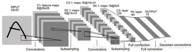
- LeNet是卷积神经网络的祖师爷LeCun在1998年提出,用于解决手写数字识别的视觉任务。自那时起,CNN的最基本的架构就定下来了:卷积层、池化层、全连接层。如今各大深度学习框架中所使用的LeNet都是简化改进过的LeNet-5(-5表示具有5个层)。和原始的LeNet有些许不同,比如把激活函数改为了现在很常用的ReLu。
- 输入尺寸为32 * 32 * 1大小,通道不限,输出为10分类任务。其模型有近五万个参数。
import torch
import torch.nn as nn

# LeNet5网络结构共5层
class LeNet5(nn.Module):
  def __init__(self):
    super(LeNet5,self).__init__()
    # in_channel,out_channel,kernel_size
    self.conv1 = nn.Conv2d(1,6,5)
    self.max_pool1 = nn.MaxPool2d((2,2),2)
    self.conv2 = nn.Conv2d(6,12,5)
    self.max_pool2 = nn.MaxPool2d((2,2),2)
    self.conv3 = nn.Conv2d(12,120,5)
    self.linear1 = nn.Linear(120,84)
    self.linear2 = nn.Linear(84,10)

  def forward(self,x):
    x = self.conv1(x)
    x = self.max_pool1(x)
    x = torch.relu(x)
    x = self.conv2(x)
    x = self.max_pool2(x)
    x = torch.relu(x)
    x = self.conv3(x)
    # print (x.shape) [None, 120, 1, 1]
    x = x.view(x.size(0),-1)
    x = self.linear1(x)
    x = self.linear2(x)
    return x
model = LeNet5()
# 如下,计算网络参数共有多少
sum(param.numel() for param in model.parameters())
Alexnet
特点:
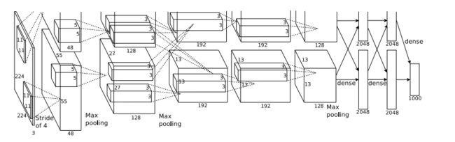
- AlexNet共包含5层卷积层和三层全连接层,层数比LeNet多了不少,但卷积神经网络总的流程并没有变化,只是在深度上加了不少。 网络大约有6千万个参数,其中3千万全用在第一个全连接层上了。
- 该网络是2012年的ImageNet竞赛中取得冠军的一个模型。模型参加的竞赛是ImageNet LSVRC-2010,该ImageNet数据集有1.2 million幅高分辨率图像,总共有1000个类别。
- 输入224 * 224 * 3大小,输出1000个类别。
看过去如下网络很复杂呀,需要怎么理解好呢?首先这幅图分为上下两个部分的网络,论文中提到这两部分网络是分别对应两个GPU,只有到了特定的网络层后才需要两块GPU进行交互,这种设置完全是利用两块GPU来提高运算的效率,其实在网络结构上差异不是很大。如下会按照一个GPU的情况编写代码。
import torch
import torch.nn as nn

class Alexnet(nn.Module):
  def __init__(self):
    super(Alexnet,self).__init__()
    # in_channel,out_channel,kernel_size
    self.lrn = nn.LocalResponseNorm(2)
    self.relu = nn.ReLU()
    self.max_pool = nn.MaxPool2d(3,stride=2)
    self.drop = nn.Dropout(p=0.5)

    self.conv1 = nn.Conv2d(3,96,11,stride=4,padding=2)
    self.conv2 = nn.Conv2d(96,256,5,stride=1,padding=2)
    self.conv3 = nn.Conv2d(256,384,3,padding=1)
    self.conv4 = nn.Conv2d(384,384,3,padding=1)
    self.conv5 = nn.Conv2d(384,256,3,padding=1)

    # 任务不同如下的linear里面的神经元的个数需要改动
    self.linear1 = nn.Linear(6*6*256,4096)
    self.linear2 = nn.Linear(4096,4096)
    self.linear3 = nn.Linear(4096,1000)
  def forward(self,x):
    x = self.max_pool(self.lrn(self.relu(self.conv1(x))))
    x = self.max_pool(self.lrn(self.relu(self.conv2(x))))
    # 第三与第四卷积层没有lrn与max_pool
    x = self.relu(self.conv3(x))
    x = self.relu(self.conv4(x))
    x = self.max_pool(self.lrn(self.relu(self.conv5(x))))
    x = x.view(x.size(0),-1)
    x = self.drop(self.relu(self.linear1(x)))
    x = self.drop(self.relu(self.linear2(x)))
    x = self.relu(self.linear3(x))
    return x
VGG
特点:
- VGGNet是牛津大学计算机视觉组和DeepMind公司共同研发一种深度卷积网络,并且在2014年在ILSVRC比赛上获得了分类项目的第二名和定位项目的第一名。
- VGG最大的贡献就是证明了卷积神经网络的深度增加和小卷积核的使用对网络的最终分类识别效果有很大的作用。
- 如下图所示,VGGNet一共有六种不同的网络结构(A、A-LRN、B、C、D、E),这6种网络结构相似,都是由5层卷积层、3层全连接层组成,其中区别在于每个卷积层的子层数量不同,从A至E依次增加(子层数量从1到4),总的网络深度从11层到19层。
- 以下会复现VGG16的代码。 VGG16输入大小为224 * 224 * 3,输出为1000个类别。其模型有1.38亿个参数,也就是138M个参数。

class VGG16(nn.Module):
  def __init__(self):
    super(VGG16,self).__init__()
    # 共五个大层卷积层,大层里面有1-3个小层
    # 由于VGG所有padding都为1,卷积核大小都是3,故使用循环构建
    self.layers = self.make_layers([64,64,'M',128,128,'M',256,256,256,'M',512,512,512,'M',512,512,512,'M'])
    self.linear1 = nn.Linear(512*7*7,4096)
    self.linear2 = nn.Linear(4096,4096)
    self.linear3 = nn.Linear(4096,1000)
  def make_layers(self,layer_info):
    layer = []
    in_channel = 3
    for info in layer_info:
      if info == 'M':
        layer.append(nn.MaxPool2d(2,2))
      else:
        layer.append(nn.Conv2d(in_channel,info,3,padding=1))
        layer.append(nn.ReLU(inplace=True))
        in_channel = info
    return nn.Sequential(*layer)

  def forward(self,x):
    x = self.layers(x)
    x = x.view(x.size(0),-1)
    x = self.linear1(x)
    x = self.linear2(x)
    x = self.linear3(x)

    return x
Google Inception
特点:
- Google Inception Net在2014年的Imagenet ILSVRC中取得第一名,该网络以结构上的创新取胜,通过采用全局平均池化层取代全连接层,极大的降低了参数量,是非常实用的模型,一般称该网络模型为Inception V1。
- 一个Inception模块,大概长如下图样子。大概参数有5M左右。代码过长,太难搞了,细节自己研究去吧【狗头保命】。

ResNet
特点:
- ResNet在2015年被提出,在ImageNet比赛classification任务上获得第一名,因为它“简单与实用”并存,之后很多方法都建立在ResNet50或者ResNet101的基础上完成的。
- 首先,ResNet在PyTorch的官方代码中共有5种不同深度的结构,深度分别为18、34、50、101、152(各种网络的深度指的是“需要通过训练更新参数”的层数,如卷积层,全连接层等),和论文完全一致。如下图是论文里给出每种ResNet的具体结构。如果论文需要对比实验,建议直接使用torchvision库里的模型。
- 如下给出resnet18的torch代码,输入为224 * 224 *3 ,输出为1000个类。其模型参数大约有11M。

class ResNet18(nn.Module):
  def __init__(self):
    super(ResNet18,self).__init__()
    self.conv1 = nn.Sequential(nn.Conv2d(3,64,kernel_size=7,stride=2,padding=3),nn.MaxPool2d(kernel_size=3,stride=2,padding=1))
    self.conv2 = nn.Sequential(BasicBlock(64,64,stride=1),BasicBlock(64,64,stride=1))
    self.conv3 = nn.Sequential(BasicBlock(64,128,stride=2),BasicBlock(128,128,stride=1))
    self.conv4 = nn.Sequential(BasicBlock(128,256,stride=2),BasicBlock(256,256,stride=1))
    self.conv5 = nn.Sequential(BasicBlock(256,512,stride=2),BasicBlock(512,512,stride=1))
    self.avg_pool = nn.AdaptiveAvgPool2d((1, 1))
    self.fc = nn.Linear(512,1000)
  def forward(self,x):
    x = self.conv1(x)
    x = self.conv2(x)
    x = self.conv3(x)
    x = self.conv4(x)
    x = self.conv5(x)
    x = self.avg_pool(x)
    x = x.view(x.size(0),-1)
    x = self.fc(x)
    return x

class BasicBlock(nn.Module):
  # 如果stride等于2,就说明要进行下采样
  def __init__(self,in_channel,out_channel,stride=1):
    super(BasicBlock,self).__init__()
    if stride == 2:
      self.downsample = nn.Conv2d(in_channel,out_channel,kernel_size=1,stride=stride)
    else:
      self.downsample = None
    self.relu = nn.ReLU(inplace=True)
    self.conv1 = nn.Conv2d(in_channel,out_channel,kernel_size=3,padding=1,stride=stride)
    self.conv2 = nn.Conv2d(out_channel,out_channel,kernel_size=3,padding=1,stride=1)
  def forward(self,x):
    x_add = x
    out = self.relu(self.conv1(x))
    out = self.relu(self.conv2(out))
    if self.downsample is not None:
      x_add = self.downsample(x)
    out += x_add
    return out
DenseNet
特点:
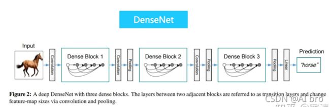
- 在残差网络之后,又出现了密集网络DenseNet(CVPR2017年的Best Paper)。它脱离了加深网络层数(ResNet)和加宽网络结构(Inception)来提升网络性能的定式思维,从特征的角度考虑,通过特征重用和旁路(Bypass)设置,既大幅度减少了网络的参数量,又在一定程度上缓解了gradient vanishing问题的产生。
- 密集网络顾名思义,它的连接更为密集,最明显的标志是密集模块即Dense Block。在Dense Block中,每一层都与其他层”沟通“,这种密集的联系,使得信息流最大化,也实现了特征的重复利用。同时网络的每一层可以被设计得特别”窄“,即只使用了比较少的特征图,可以达到降低冗余的目的,这使得DenseNet的计算量也比较小。
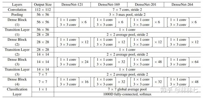
- 相比ResNet拥有更少的参数数量,如下实现DenseNet-121网络,只有大约8M个参数。输入为224 * 224 * 3,输出为1000类。
# 完成基本内容块的制作,包括输入维度,增长速率k,bn_size
# 类前面加下划线,表示此类只用于内部访问
import torch
import torch.nn as nn
import torch.nn.functional as F
from collections import OrderedDict

class _DenseLayer(nn.Sequential):
  def __init__(self,in_channel,grow_rate,bn_size):
    super(_DenseLayer,self).__init__()
    self.add_module('bn1',nn.BatchNorm2d(in_channel))
    self.add_module('relu1',nn.ReLU(inplace = True))
    self.add_module('conv1',nn.Conv2d(in_channel,bn_size*grow_rate,kernel_size=1,bias=False))
    self.add_module('bn2',nn.BatchNorm2d(bn_size*grow_rate))
    self.add_module('relu2',nn.ReLU(inplace = True))
    self.add_module('conv2',nn.Conv2d(bn_size*grow_rate,grow_rate,kernel_size=3,padding=1,bias=False))
  # 这个实际上nn.Sequential已经实现了的
  # 这里我们需要重写,使得前后相连
  def forward(self,input):
    new_feature = super(_DenseLayer,self).forward(input)
    # 在维度为1的位置将其串联起来
    return torch.cat([input,new_feature],1)

class _DenseBlock(nn.Sequential):
  def __init__(self,layer_nums,in_channel,grow_rate,bn_size):
    super(_DenseBlock,self).__init__()
    for i in range(layer_nums):
      self.add_module('layer{}'.format(i+1),_DenseLayer(in_channel+grow_rate*i,grow_rate,bn_size))
  def forward(self,input):
    for m in self:
      input = m(input)
    return input

class _TransitionLayer(nn.Sequential):
  def __init__(self,in_channel,out_channel):
    super(_TransitionLayer,self).__init__()
    self.add_module('norm', nn.BatchNorm2d(in_channel))
    self.add_module('relu', nn.ReLU(inplace=True))
    self.add_module('conv',nn.Conv2d(in_channel,out_channel,kernel_size=1,bias=False))
    self.add_module('avg_pool',nn.AvgPool2d(stride=2,kernel_size=2))
  def forward(self,input):
    for m in self:
      input = m(input)
    return input

class DenseNet121(nn.Module):
  def __init__(self,init_channel=64,grow_rate=32,bn_size=4):
    super(DenseNet121,self).__init__()
    block_list = [6,12,24,16]
    self.all_feature = nn.Sequential(OrderedDict([('conv1',nn.Conv2d(3,init_channel,kernel_size=7,stride=2,padding=3)),
                            ('bn1',nn.BatchNorm2d(init_channel)),
                            ('relu1',nn.ReLU(inplace=True)),
                            ('max_pool1',nn.MaxPool2d(kernel_size=3,stride=2,padding=1))]
                            ))
    cur_channel = init_channel
    for i,block_num in enumerate(block_list):
      self.all_feature.add_module('DenseBlock{}'.format(i+1),_DenseBlock(block_num,cur_channel,grow_rate,bn_size))
      cur_channel = cur_channel + grow_rate*block_num
      if i != len(block_list)-1:
        self.all_feature.add_module('Transition{}'.format(i+1),_TransitionLayer(cur_channel,cur_channel//2))
        # print (cur_channel)
        # 使用//是因为,保证通道数为整数
        cur_channel = cur_channel//2
        # print (cur_channel)

    self.classifier = nn.Linear(cur_channel,1000)

  def forward(self,x):
    x = self.all_feature(x)
    x = F.relu(x,inplace=True)
    x = F.avg_pool2d(x,kernel_size=7)
    x = x.view(x.size(0),-1)
    x = self.classifier(x)
    return x
# DenseNet121()
参考资料:
具体网络结构详情,可见如下链接:
AlexNet:https://blog.csdn.net/luoluonuoyasuolong/article/details/81750190
VGG:https://blog.csdn.net/daydayup_668819/article/details/79932324
ResNet:https://zhuanlan.zhihu.com/p/79378841
ResNet:https://www.jianshu.com/p/085f4c8256f1
DenseNet:https://zhuanlan.zhihu.com/p/67311529
DenseNet:https://zhuanlan.zhihu.com/p/43057737
DenseNet:https://www.cnblogs.com/lyp1010/p/11820967.html
Google Inception:https://www.jianshu.com/p/680645517020
Google Inception:https://blog.csdn.net/sinat_29957455/article/details/80766850
代码汇总:
https://colab.research.google.com/drive/1mAcCzTb038-NuQ8IGDHmeWqGSzO3z7R4?usp=sharing