python复现:PCA-based spatially adaptive denoising of CFA images for single-sensor digital cameras
PCA-based spatially adaptive denoising of CFA images for single-sensor digital cameras
是2009年一篇基于PCA的图像降噪方法,应用在raw图上,下面的代码和
官方 matlab的结果是一致的(因为是逐句翻译的、、、),但是效率很低,优化空间很大,比如取patch的时候重复计算了很多次。
import cv2
import matplotlib.pyplot as plt
import numpy as np
import scipy
import scipy.signal

# 各通道噪声方差
from colour_demosaicing import demosaicing_CFA_Bayer_bilinear
%matplotlib inline
file = r'kodak_fence.tif'
im = cv2.imread(file)
im = im[..., :3]
im = im[..., ::-1]
print(im[100:110,100:110,-1])
[[124 126 128 123 121 121 114 117 122 115]
 [127 128 127 123 121 119 119 120 117 117]
 [127 127 124 124 121 121 120 118 118 112]
 [124 123 119 123 120 121 118 116 117 115]
 [120 115 116 119 121 119 116 114 113 111]
 [119 120 120 122 120 118 111 113 114 113]
 [123 120 121 122 116 115 109 111 118 114]
 [125 123 120 119 117 113 114 113 116 114]
 [117 119 121 119 120 114 115 113 117 116]
 [118 119 120 121 119 118 114 113 118 116]]
im2 = cv2.imread('noise.png')[...,::-1]
im_noise=im2.copy()
print(im2[100:110,100:110,-1])
[[129 127 104 134 132 116 108 108 107 119]
 [146 130 134 122 127 128 116 117 123 119]
 [118 139 125 128 120 113 125 120 138 121]
 [128 133 125 122 116 116 109 114 101 103]
 [110 117 115 116 125 121 124 109 118 117]
 [118 101 130 126 105 118 122 118 108 104]
 [115 116 129  98 119  87 107 106 115 117]
 [124 123 114 109 129 111 120 132 114  97]
 [121 112 134 102  99 130 124 130 130 102]
 [121 112 112 127 106 125 118  98 135 135]]
im.shape
im_clean=im.copy()
bb=1
psnr_noise = 10 * np.log10(255 ** 2 / np.mean((im[bb:-bb,bb:-bb] - im_noise[bb:-bb,bb:-bb]) ** 2, axis=(0,1)))
print(psnr_noise)
[ 29.57315911 29.71359964 30.30441583]
def black_sub(filename, height=800, width=800):
    raw_image = np.fromfile(filename, dtype=np.uint16)
    print(len(raw_image))
    raw_image = raw_image.reshape([height, width])

    # black level
    black_level = 16
    white_level = 1023
    normalized_image = raw_image.astype(np.float32) - black_level
    # if some values were smaller than black level
    normalized_image[normalized_image < 0] = 0
    normalized_image = normalized_image / (white_level - black_level)

    print(normalized_image.min(), normalized_image.max())

    normalized_image = normalized_image * 255
    normalized_image2 = np.clip(normalized_image, 0, 255).astype(np.uint8)
    return normalized_image2
# filename = r'D:\dataset\dang_yingxiangzhiliangceshi\raw\cap_frame_3641.raw'
# tI = black_sub(filename, height=800, width=800)

# mI=cv2.blur(tI, (30,30))
n, m, ch = im.shape

mI=np.zeros([n, m])
tI=np.zeros([n, m])

# noise grgb
mI[0:n,0:m] = im2[:,:,1]
mI[0:n:2,1:m:2] = im2[0:n:2,1:m:2, 0]
mI[1:n:2,0:m:2] = im2[1:n:2,0:m:2, 2]

tI[0:n,0:m] = im[:,:,1]
tI[0:n:2,1:m:2] = im[0:n:2,1:m:2, 0]
tI[1:n:2,0:m:2] = im[1:n:2,0:m:2, 2]
psnr = 10 * np.log10(255 ** 2 / np.mean(((mI - tI) ** 2)))
print(psnr)
26.7146060444
2. decomposition
def get_gauss(sigma, len):
    x = np.arange(-len,len+1)
    y = np.arange(-len,len+1)
    xx, yy = np.meshgrid(x,y)
    z = np.exp(-(xx*xx+yy*yy)/2/(sigma*sigma)) / (2 * np.pi * sigma*sigma)
    return z

w = 10
f = get_gauss(3, w)
print(f[:10,:10])
[[  2.64291611e-07   7.59460747e-07   1.95286554e-06   4.49349653e-06
    9.25212596e-06   1.70468335e-05   2.81054770e-05   4.14651518e-05
    5.47419944e-05   6.46700251e-05]
 [  7.59460747e-07   2.18236448e-06   5.61169806e-06   1.29123819e-05
    2.65866421e-05   4.89852888e-05   8.07630877e-05   1.19153063e-04
    1.57305015e-04   1.85833918e-04]
 [  1.95286554e-06   5.61169806e-06   1.44298331e-05   3.32026980e-05
    6.83644778e-05   1.25960009e-04   2.07672947e-04   3.06388333e-04
    4.04491667e-04   4.77850443e-04]
 [  4.49349653e-06   1.29123819e-05   3.32026980e-05   7.63986075e-05
    1.57305015e-04   2.89830945e-04   4.77850443e-04   7.04992167e-04
    9.30725575e-04   1.09952235e-03]
 [  9.25212596e-06   2.65866421e-05   6.83644778e-05   1.57305015e-04
    3.23891607e-04   5.96762985e-04   9.83895828e-04   1.45158148e-03
    1.91636740e-03   2.26392058e-03]
 [  1.70468335e-05   4.89852888e-05   1.25960009e-04   2.89830945e-04
    5.96762985e-04   1.09952235e-03   1.81280588e-03   2.67450615e-03
    3.53086373e-03   4.17122264e-03]
 [  2.81054770e-05   8.07630877e-05   2.07672947e-04   4.77850443e-04
    9.83895828e-04   1.81280588e-03   2.98881162e-03   4.40951518e-03
    5.82141014e-03   6.87718348e-03]
 [  4.14651518e-05   1.19153063e-04   3.06388333e-04   7.04992167e-04
    1.45158148e-03   2.67450615e-03   4.40951518e-03   6.50553684e-03
    8.58856282e-03   1.01461881e-02]
 [  5.47419944e-05   1.57305015e-04   4.04491667e-04   9.30725575e-04
    1.91636740e-03   3.53086373e-03   5.82141014e-03   8.58856282e-03
    1.13385587e-02   1.33949244e-02]
 [  6.46700251e-05   1.85833918e-04   4.77850443e-04   1.09952235e-03
    2.26392058e-03   4.17122264e-03   6.87718348e-03   1.01461881e-02
    1.33949244e-02   1.58242334e-02]]
w = 10

fmI = cv2.GaussianBlur(mI,(2*w+1,2*w+1),3)
print(fmI[100:110,100:110])
[[ 121.93832694  120.80475462  119.34427302  117.70715601  116.06921131
   114.58486129  113.35933285  112.43633939  111.81440447  111.46699312]
 [ 121.52631498  120.47457756  119.06497391  117.42939834  115.73886432
   114.16113306  112.82476593  111.80118861  111.11348537  110.74756437]
 [ 120.87684224  119.92483971  118.59186934  116.98478683  115.2656273
   113.61417197  112.18455321  111.07980339  110.35132867  109.99891044]
 [ 120.06088905  119.22871398  118.0002417   116.45487617  114.74288424
   113.05241178  111.56081857  110.40168771  109.65525121  109.33631585]
 [ 119.17015693  118.48072734  117.38722186  115.94233693  114.28226138
   112.59720486  111.08110038  109.89275087  109.13933657  108.8525714 ]
 [ 118.2985367   117.77233662  116.84362262  115.54084722  113.98304615
   112.35314865  110.851063    109.65205922  108.88682568  108.60707037]
 [ 117.48539156  117.12919512  116.38418959  115.25858743  113.85106686
   112.32643485  110.8775763   109.68491146  108.89737908  108.58942516]
 [ 116.73276808  116.52954776  115.9655374   115.0346916   113.81328909
   112.43786173  111.08081869  109.91515716  109.10092106  108.73597896]
 [ 115.98315995  115.88488868  115.46792689  114.72136547  113.70067514
   112.5076856   111.28264307  110.17813221  109.35522429  108.93094655]
 [ 115.16712536  115.10319425  114.77481649  114.17840339  113.35413192
   112.36733278  111.31740348  110.32423396  109.53731509  109.08319369]]
smI = mI - fmI
print(smI[100:110,100:110])
[[ 29.06167306  12.19524538 -14.34427302 -16.70715601 -10.06921131
   17.41513871  -5.35933285  17.56366061  -5.81440447  -5.46699312]
 [ 24.47368502  27.52542244  14.93502609 -13.42939834  11.26113568
  -14.16113306   3.17523407   0.19881139  11.88651463  -1.74756437]
 [  6.12315776  -2.92483971  21.40813066  13.01521317   9.7343727
    7.38582803 -11.18455321 -13.07980339 -13.35132867  14.00108956]
 [  7.93911095 -17.22871398   6.9997583   -5.45487617   1.25711576
  -10.05241178  -2.56081857  -4.40168771  -8.65525121 -14.33631585]
 [-14.17015693  -1.48072734   2.61277814 -15.94233693  -4.28226138
   -3.59720486   9.91889962   2.10724913 -10.13933657  21.1474286 ]
 [ -0.2985367   12.22766338  13.15637738  29.45915278  -8.98304615
   -7.35314865  11.148937   -20.65205922  -0.88682568  17.39292963]
 [  4.51460844   0.87080488  -0.38418959   1.74141257 -25.85106686
  -25.32643485 -21.8775763  -37.68491146   4.10262092 -36.58942516]
 [  7.26723192  -3.52954776  -1.9655374    6.9653084   15.18671091
   -1.43786173   8.91918131 -13.91515716   4.89907894   9.26402104]
 [-11.98315995  14.11511132   9.53207311  23.27863453  -7.70067514
   17.4923144   10.71735693   8.82186779   5.64477571  -3.93094655]
 [  5.83287464  -5.10319425  -2.77481649  14.82159661  -7.35413192
   29.63266722   6.68259652 -22.32423396  25.46268491  -3.08319369]]
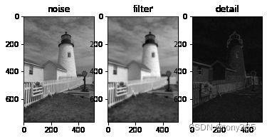
plt.figure()
plt.subplot(131)
plt.imshow(mI, cmap='gray')
plt.title("noise")
plt.subplot(132)
plt.imshow(fmI, cmap='gray')
plt.title("filter")
plt.subplot(133)
plt.imshow(np.abs(smI), cmap='gray')
plt.title("detail")
plt.show()
denoiseing
dI=smI.copy();
s=6;#default variable block size
k=34;# training block size,(k-s)/2 should be an even integer%%%%%%%%%
k2=k//2;

#Bayer Pattern: G R; B G
v=12;
vr=13/12;
vb=10/12;
vg=1;


# noise pattern, GRBG的6*6,每个通道的噪声方差乘上一个 1.21倍
c=1.1
D = np.zeros([s,s], dtype=np.float32)
D[:,:] = c*vg*v
D[0:s:2, 1:s:2] = c*vr*v  # r
D[1:s:2, 0:s:2] = c*vb*v  # b
D=D**2
print(D)
[[ 174.23999  204.49     174.23999  204.49     174.23999  204.49   ]
 [ 121.       174.23999  121.       174.23999  121.       174.23999]
 [ 174.23999  204.49     174.23999  204.49     174.23999  204.49   ]
 [ 121.       174.23999  121.       174.23999  121.       174.23999]
 [ 174.23999  204.49     174.23999  204.49     174.23999  204.49   ]
 [ 121.       174.23999  121.       174.23999  121.       174.23999]]
def get_pca(X, D):
    """
    X : 36 * 100 , fetures * n_samples
    D : 36, 每个feature的噪声方差
    """
    D = D.reshape(-1)
    h, n = X.shape
    mx = np.mean(X, 1).reshape(-1, 1)
    X = X - mx

    convX = X @ X.T / (n-1)

    DD = np.diag( D)


    convX = convX - DD

    convX[convX < 0] = 0.0001

    [eig_val, eig_vec] = np.linalg.eigh(convX) # convX * eig_vec = eig_val.reshape(1, -1) * eig_vec
    # eig_val是特征值, eig_vec是对应的特征向量,col形式的。
    #print('eig_val : ', eig_val,eig_vec, eig_val.shape, eig_vec.shape)
    # print(np.sum(convX @ eig_vec - eig_val.reshape(1, -1) * eig_vec <0.01))
    # print(eig_vec @ X == X @eig_vec.T)
    ind = np.argsort(eig_val)
    ind = ind[::-1]

    eig_vec = eig_vec[:,ind].T
    eig_val = eig_val[ind]

    Y = eig_vec @ X
    #print('ind:\n',ind, eig_val,eig_vec ,Y)

    return Y, eig_vec, eig_val, mx
tttt=0

def pca_cfa(block, D, s):
    global tttt
    """
    block : 34*34 block, k = 34
    D:
    s:6 or 8
    """
    h, w = block.shape
    H = (h-s) // 2 + 1 # 15
    W = (w-s) // 2 + 1
    L = H*W

    X = np.zeros([s*s, L]) # 36*225 : 34*34的block, 6*6的patch, step为2, 一共15*15=225个patch

    DN = np.zeros([1, s*s])

    k = 0
    for i in np.arange(0, s):
        for j in np.arange(0, s):

            X[k, :] = block[i:(h-s+i+1):2, j:(w-s+j+1):2].reshape([1, L])
            DN[0, k] = D[i, j]
            k = k + 1
    # X是 6*6 * 225
    # DN 是 6*6个值,每个值对应的该像素的标准差
    # 中间的一个值
    q = L // 2 # 112
    Xc = X[:, q].reshape(-1, 1) # 36
    XC = np.tile(Xc, [1, L]) # 36 * 225

    # print(DN, k, X.shape, XC.shape)

    E = np.abs(X-XC)
    mE = np.mean(E, axis=0) # 每列的均值,相当于求每个patch与中心patch的均值

    ind = np.argsort(mE)
    num = 100
    X = X[:, ind[:num]]
    # print('X:',X[:10,:10], DN)
    # 到这里选出了100个相似的patch, 从225个里面
    Y, P, V, mx = get_pca(X, DN)
    #print(Y[:10,:10])
    Y1 = np.zeros(Y.shape)

    # inverse transform\
    # (设置10个为0)
    for i in np.arange(0,s*s-8):
        y = Y[i,:]
        p = P[i,:]
        p = p*p

        nv = np.sum(p*DN) # p*DN 噪声方差经过 pca转置, P是单位矩阵,类似求均值了,所以sum

        if 0==tttt:
            print(p.shape, DN.shape, (p*DN).shape,nv.shape)
        py = np.mean(y*y) + 0.01

        t = max(0, py-nv)
        if 0==tttt:
            print(py.shape,py, t)
            tttt = 1
        c = t / py
        # print(c) #基本上很小的数,0-0.3之间
        Y1[i, :] = 1* Y[i, :]


    B = P.T @ Y1 + mx
    B = B[:, 0]
    B = np.reshape(B, [s, s])
    #B = B.T
    return B
step = 2
print(n-k,m-k)
for i in np.arange(0, n - k, step):
    for j in np.arange(0, m - k, step):
        #if i== 50 and j==50:
            Block = smI[i:i+k, j:j+k].copy()
            db = pca_cfa(Block, D, s)
            dI[i+k2-1:i+k2+1, j+k2-1:j+k2+1] = db[2:4, 2:4]
            #print(Block[:10,:10])
            #print(db)
            #print(x[:10.:10])
            #print(y[:10.:10])
734 478
(36,) (1, 36) (1, 36) ()
() 167.639940721 0
i
a = n-k
b=i+k-1
c=i+k2-1
db
t = dI[99:110,99:110]
print(i,a,b,c,db,t)
732 734 765 748 [[-25.80532161  11.18396885  21.5562875   15.1691311   15.48400112
   29.98028105]
 [-26.3432829   21.56501168 -43.50587703   4.79103188  -4.43557792
   -7.3855937 ]
 [ 17.00578207  57.53942483  28.85620708  29.88176839  15.84105093
   13.18102019]
 [-25.43627059  22.4839088   16.93029056  14.54577497 -20.64510537
   -5.64869904]
 [  0.15234094  -5.87031587   9.84325354  21.98484204  -6.78422562
   30.82852626]
 [ -2.9422656   -5.54282893 -14.33997315  -2.43183229 -39.36737168
   14.82723805]] [[  2.39425621  -7.50795736  10.1263103   -1.00761166 -14.14296723
    4.27147071   9.48992787 -17.40794547   8.14357609  -0.59332369
    1.87093838]
 [ -5.92387084  31.39388273  14.87143502 -12.58273904 -11.87516387
   -2.60759948   8.9776016   -4.55399497  11.75790601  -5.73767096
   -6.51739886]
 [  6.10456174  22.48420321  21.68501677  15.79794982 -15.88482472
   11.86451625  -9.66591387   3.03897717   2.02633336  12.9747562
    1.73978256]
 [ -7.54473426  10.60003328   4.92408636  18.46661195   8.99161538
    6.65299865   5.16234318 -15.96123275  -7.76966259 -13.20031974
    2.27381012]
 [-16.26497218   2.37717583 -22.06340946   0.59562629  -5.18313707
    4.26679605 -17.48835341   2.85138918  -4.56904362  -9.51967616
  -15.8008651 ]
 [  0.70260208   1.76680755   2.85435522  -2.78418131  -7.97310004
   -2.99846244  -3.51906016   9.60667614   3.02749668   3.41880403
   22.40951242]
 [  2.06235778  -0.97282281   8.61112305  18.59272929  28.4612208
   -7.33356166  -5.07142281  11.37647051 -22.11546397  -7.40368596
    3.12237772]
 [ -6.29088137   2.36391139  -7.30272654   0.05294837   4.31963347
  -22.88124845 -27.44595565 -21.358552   -36.03650032  12.40441245
  -30.47078166]
 [  6.96705517   4.26531585   3.541887     1.30659318   3.03703037
   15.66634705  -2.43022019   6.90065626 -13.58299795   5.86283103
   10.24549084]
 [  8.18625562  -4.30581833   7.32269359   9.17154543  21.27121419
   -2.85394241  19.95621912   7.63124297   3.05477624   4.34158611
   -9.33247657]
 [ -4.23236535  10.92552271  -9.23752909  -0.75844497  16.45297477
   -4.0952441   29.42888478   7.88977393 -17.74546651  23.72911602
   -0.42439872]]
ddI = dI.copy()

ddI = ddI + fmI

plt.figure(figsize=(20,15))
plt.subplot(131)
plt.imshow(mI,cmap='gray')
plt.subplot(132)
plt.imshow(tI,cmap='gray')
plt.subplot(133)
plt.imshow(ddI,cmap='gray')
plt.show()
bb = 20
psnr = 10 * np.log10(255 ** 2 / np.mean(((ddI[bb:-bb,bb:-bb] - tI[bb:-bb,bb:-bb]) ** 2)))
print(psnr)
psnr = 10 * np.log10(255 ** 2 / np.mean(((mI[bb:-bb,bb:-bb] - tI[bb:-bb,bb:-bb]) ** 2)))
print(psnr)
27.4094591896
26.7145989939
print(ddI.min(),ddI.max(),ddI.mean())
#
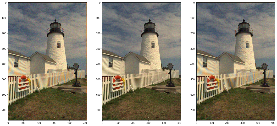
im_noise_bayer2rgb = demosaicing_CFA_Bayer_bilinear(mI, "GRBG")
im_noise_bayer2rgb2 = np.clip(im_noise_bayer2rgb,0,255).astype(np.uint8)
rgb = demosaicing_CFA_Bayer_bilinear(ddI, "GRBG")
rgb2 = np.clip(rgb,0,255).astype(np.uint8)
print(rgb2.max(),rgb2.min())
plt.figure(figsize=(20,15))
plt.subplot(131)
plt.imshow(im_noise_bayer2rgb2)
plt.subplot(132)
plt.imshow(im2)
plt.subplot(133)
plt.imshow(rgb2)
plt.show()
bb = 1
psnr = 10 * np.log10(255 ** 2 / np.mean(((im[bb:-bb,bb:-bb] - rgb2[bb:-bb,bb:-bb]) ** 2)))
print(psnr)
psnr_noise = 10 * np.log10(255 ** 2 / np.mean(((im[bb:-bb,bb:-bb] - im2[bb:-bb,bb:-bb]) ** 2)))
print(psnr_noise)
bb = 1
psnr = 10 * np.log10(255 ** 2 / np.mean(((im[bb:-bb,bb:-bb] - rgb2[bb:-bb,bb:-bb]) ** 2), axis=(0,1)))
print(psnr)
psnr_noise = 10 * np.log10(255 ** 2 / np.mean(((im[bb:-bb,bb:-bb] - im_noise[bb:-bb,bb:-bb]) ** 2), axis=(0,1)))
print(psnr_noise)
-13.911260205 273.354212873 112.224014452
255 0
30.3929142051
29.8523440731
[ 30.19659709 30.45414954 30.53523719]
[ 29.57315911 29.71359964 30.30441583]
bayer_diff_noise = np.abs(im_noise_bayer2rgb-im2)
bayer_diff_noise2 = np.clip(bayer_diff_noise,0,255).astype(np.uint8)+40
plt.figure(figsize=(20,15))
plt.imshow(bayer_diff_noise2)
plt.show()

bayer_diff_denoise = np.abs(im_noise_bayer2rgb-rgb2)
bayer_diff_denoise2 = np.clip(bayer_diff_noise,0,255).astype(np.uint8)+40
plt.figure(figsize=(20,15))
plt.imshow(bayer_diff_denoise2)
plt.show()
q = np.random.randn(18,6)
conv = q.T@q
[eig_val, eig_vec] = np.linalg.eigh(conv)
# convX * eig_vec = eig_val.reshape(1, -1) * eig_vec
# eig_val是特征值, eig_vec是对应的特征向量,col形式的。
print('eig_val : ', eig_val,eig_vec, eig_val.shape, eig_vec.shape)
print(np.sum(conv @ eig_vec - eig_val.reshape(1, -1) * eig_vec <0.01))
print(eig_vec @ conv - (conv @eig_vec.T).T)
print(q @ eig_vec.T , (eig_vec.T @ q.T).T)
print(eig_vec @ conv)
eig_val :  [  3.00685873   6.20435828  11.58297164  13.42519523  17.63008572
  43.47319024] [[ 0.08787425 -0.32322719  0.68824544 -0.17445992  0.61739305 -0.05010059]
 [ 0.20655283 -0.32032156 -0.31217256 -0.10821841  0.05036977 -0.86199187]
 [-0.39190487 -0.22314618 -0.36999561 -0.7642356   0.15395569  0.22794997]
 [-0.02485003  0.34875418 -0.446504    0.2923101   0.76925841  0.03440172]
 [-0.34883424 -0.73228301 -0.1652491   0.53024788  0.01514715  0.18269308]
 [-0.82080556  0.29198661  0.25553213  0.08478473 -0.0244625  -0.40980303]] (6,) (6, 6)
36
[[ 0.  0.  0.  0.  0.  0.]
 [ 0.  0.  0.  0.  0.  0.]
 [ 0.  0.  0.  0.  0.  0.]
 [ 0.  0.  0.  0.  0.  0.]
 [ 0.  0.  0.  0.  0.  0.]
 [ 0.  0.  0.  0.  0.  0.]]
[[-0.28604411 -1.12444082 -1.99047454 -0.81004248 -1.61292579 -0.66351663]
 [ 0.21973116  0.35220044  0.2430437  -0.22633582  0.70423737 -1.21817532]
 [-0.48757707  0.01916215  0.15872299 -0.52964081  1.14307178 -0.31505747]
 [-1.30867509 -0.36797715 -0.33869114  1.48919373  0.25654388 -0.5580843 ]
 [ 0.95980308 -0.3433002   0.48891304  1.65378029  0.9426408   0.79037999]
 [-0.82253679 -0.4499282  -1.73138871  1.46541122  0.29257894 -0.12554285]
 [-0.57803434 -0.12893755  0.97914154  1.18823126 -1.00594376  0.42347444]
 [ 0.93968361  0.86445293 -1.43869371 -0.24434619  1.03763686  0.05760273]
 [ 0.61635883  1.11112675 -0.07769851 -0.49675303  1.05073505 -0.5592649 ]
 [-2.18383768 -2.01124521 -1.16609084  1.29879153 -1.17353974 -0.45591985]
 [-0.36399424 -0.78391182  0.35930308 -0.19128518  0.26045013 -1.02106562]
 [ 1.32562539  0.37206846 -0.69934282  0.2410139  -0.68051064 -1.20360493]
 [ 0.11779126 -0.12449757 -0.52275902 -0.22211952 -0.61323223  0.22617533]
 [-0.27327115 -0.94221235 -0.99726921 -0.05611817 -0.15930349  1.35568788]
 [ 1.39445607 -0.25021183 -0.63857315 -1.01563787  0.89414256  0.87480807]
 [-0.77712993 -1.08026094  1.29529701 -0.82567868 -0.92267392  0.13429965]
 [ 1.69804121  2.26584728 -0.53652959 -0.75482311  2.53634673  0.09713854]
 [ 0.26171984  0.42264116 -0.62067484  0.33506406  0.45127744 -1.77625057]] [[-0.05136115 -0.16015255  0.20927743 -1.91351599  1.69654497 -1.5473325 ]
 [-0.3466322   0.26303613  1.1393501   0.32727152  0.2967792   0.76149943]
 [-0.13502622  1.21278329  0.34400607  0.27365695  0.02051475  0.51668239]
 [ 0.13371458  0.34012412  0.14721203  1.53336544  0.77306548 -1.20567201]
 [-1.00318087 -0.66462649 -1.21801211  1.50908486 -0.32198251  0.46228868]
 [ 0.13852317  0.15944682 -0.74832478  1.00510857  1.87510392 -0.9973177 ]
 [ 0.35020046 -0.79061303 -0.12505924  0.82516552 -0.98020791 -1.2278269 ]
 [ 0.15218709  0.03377902 -0.56454656 -0.18720029  1.38505245  1.59480662]
 [ 0.15723072  0.22838697  0.54392109  0.14056405  0.34432641  1.66525424]
 [-0.11682554  0.47656554 -0.13409514  0.46727202  1.24691184 -3.37847056]
 [-0.77504359  0.58505138  0.93077875  0.12223913  0.05350184 -0.44269169]
 [-0.36338127 -1.44019124  0.7929206  -0.40871018  1.06776627  0.46103859]
 [ 0.16845739 -0.29130282 -0.26683035 -0.65513962  0.27303937 -0.30167113]
 [-0.06772517  0.39145899 -1.61245105 -0.5986978   0.34968528 -0.76476109]
 [-0.7802866   0.27700291 -1.11717732 -1.04000602  0.21367203  1.39651656]
 [-0.30160065  0.48566603  0.49775838 -0.75119022 -1.49195163 -1.27866865]
 [ 0.31816796  0.38629151 -0.27657952  0.33850528  0.67752998  3.79696451]
 [-0.26735673 -0.18439108  1.29255671  0.50863063  1.35019886  0.49539963]]
[[ -0.40105476 -19.20241152   9.97654104  -0.40928512   6.29898326
  -10.4763983 ]
 [  0.50257292 -20.69111949   2.49696061   0.02592651   5.38770129
  -11.44541867]
 [ -7.98031657  -3.67744296  -5.78579834 -12.84257337   1.56109153
    1.28449002]
 [ -0.2390802   10.52613786  -8.81522432   5.15695706   6.19921855
    4.25763913]
 [ -3.32536728 -22.28929842   1.40108721   6.37097294   5.42142478
   -8.08483245]
 [-11.00613909   2.56600124   3.68737603  -0.84821884   0.51813781
   -3.33330161]]