口译: (Interpreting:)
OLS (Ordinary Least Squared) Regression is the most simple linear regression model also known as the base model for Linear Regression. While it is a simple model, in Machine learning it is not given much weightage. OLS is one such model which tells you much more than only the accuracy of the overall model. It also tells you how each variables have fared, if we have unwanted variables, if there is autocorrelation in the data and so on.
OLS(普通最小二乘)回归是最简单的线性回归模型,也称为线性回归的基础模型。 尽管它是一个简单的模型,但是在机器学习中却没有太多的权重。 OLS就是这样一种模型,它告诉您的不仅是整个模型的准确性。 它还告诉您每个变量的运行情况,是否有不需要的变量,数据中是否存在自相关等。
It is also one of the easier and more intuitive techniques to understand, and it provides a good basis for learning more advanced concepts and techniques. This post explains how to perform linear regression using the statsmodels Python package.
它也是一种更容易理解,更直观的技术,并且为学习更高级的概念和技术提供了良好的基础。 这篇文章说明了如何使用statsmodels Python软件包执行线性回归。
Note: There is also a Logit Regression which is similar to Sklearn’s Logistic Regression and works for classification problems.
注意:还有一个Logit回归,类似于Sklearn的Logistic回归,适用于分类问题。
OLS reflects the relationship between X and y variables following the simple formula:
OLS按照以下简单公式反映X和y变量之间的关系:
Y = b1X +b0 #Simple Linear
Y = b1X + b0#简单线性
= b0 + b1X1 + b2X2…. + #Multi Linear
= b0 + b1X1 + b2X2…。 + #多线性
Where
哪里
· b0 — y — intercept
·b0 — y —截距
· b1,b2 — slope
·b1,b2 —斜率
· X, X1, X2 — predictor
·X,X1,X2-预测变量
· y — Target variable
·y-目标变量
OLS is an estimator in which the values of b1 and b0 (from the above equation) are chosen in such a way as to minimize the sum of the squares of the differences between the observed dependent variable and predicted dependent variable. That’s why it’s named ordinary least squares.
OLS是一种估计器,其中b1和b0的值(根据上述方程式)的选择方式应使所观察到的因变量与预测因变量之间的差平方和最小。 这就是为什么它被称为普通最小二乘法。
Also when the model is trying to reduce the error rate between predicted and actual, it means its trying to cut down on losses and predict better. You are trying to predict the impact of your predictors on the results.
同样,当模型试图降低预测和实际之间的错误率时,这意味着它试图减少损失并更好地进行预测。 您正在尝试预测预测变量对结果的影响。
Note: Ideally before computing the model building using OLS, the linear assumptions need to be met. The aim of this article is to interpret all the elements in an OLS model.
注意:理想情况下,在使用OLS计算模型构建之前,需要满足线性假设。 本文的目的是解释OLS模型中的所有元素。
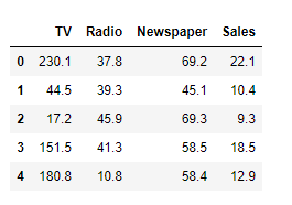
Lets understand this better looking at this example, I have taken a simple dataset — Advertising data:
让我们通过下面的示例更好地了解这一点,我采用了一个简单的数据集-广告数据:
Data in consideration. Data shape is 200x4 考虑数据。 数据形状为200x4In linear models, the coefficient of 1 variable is dependent on other independent variables. Hence if there is a reduction or addition in the data, it will affect the whole model. For example, suppose in the future, we also have another advertising medium say Social Media, we will have to re-fit and re-calculate the coefficients and the constants as they are dependent on dimensions of the dataset.
在线性模型中,1变量的系数取决于其他自变量。 因此,如果数据减少或增加,则会影响整个模型。 例如,假设在将来,我们还有另一种广告媒体,例如“社交媒体”,我们将不得不重新拟合和重新计算系数和常数,因为它们取决于数据集的维数。
In case you want to check out the formula for multi linear regression:
如果您想查看用于多元线性回归的公式:
So practically, it’s not feasible to keep adding variables and checking their linear relationship. The idea is to pick the best of variables using the following 2 steps:
因此,实际上,不断添加变量并检查它们的线性关系是不可行的。 这个想法是通过以下两个步骤来选择最佳变量:
1. Domain Knowledge
1.领域知识
2. Statistical tests — Not only the parametric and non-parametric tests but also check if there is multicollinearity between independent variables and correlation with target variables.
2.统计检验-不仅要进行参数检验和非参数检验,还要检查自变量与目标变量之间的相关性是否存在多重共线性。
Heatmap for correlation 相关热图Here we quickly check the correlation for the data and its evident that Sales and TV advertising has a strong correlation. Say for example, an increase in Advertising leads to an increase in Sales, however if a medium like Newspaper has a low readership, it may also lead to a negative correlation.
在这里,我们快速检查了数据的相关性,并证明了销售和电视广告具有很强的相关性。 举例来说,广告的增加会导致销售量的增加,但是,如果像报纸这样的媒体的读者人数较少,那么这也可能导致负相关。
Thus getting our variables right is the most important step for any model building. This will help reduce processing costs while building the right Machine Learning models.
因此,正确设置变量是任何模型构建中最重要的步骤。 这将有助于在构建正确的机器学习模型时降低处理成本。
Step 1: Import the libraries and add a constant element. We do so because we expect our dependent variables to take a non-zero value when all the other included regressors are set to zero. This value would show up as a constant i.e. 1. Later when we form the model, the coefficient of the constant value will be b0 in our multi linear formula.
步骤1:导入库并添加一个常量元素。 这样做是因为当所有其他包含的回归变量都设置为零时,我们期望我们的因变量采用非零值。 该值将显示为常数,即1。稍后,当我们形成模型时,常数值的系数在我们的多元线性公式中为b0。
X variables with constant X个常数变量Step 2: Fit the X and y variables and check the summary. Now let’s run and have a look at the results. We will interpret each and every section of this summary table.
步骤2:拟合X和y变量并检查摘要。 现在开始运行,看看结果。 我们将解释此汇总表的每个部分。
OLS model OLS模型For easy explanation purposes, we will divide the summary report into 4 sections.
为了便于说明,我们将摘要报告分为四个部分。
SECTION 1:
第1节:
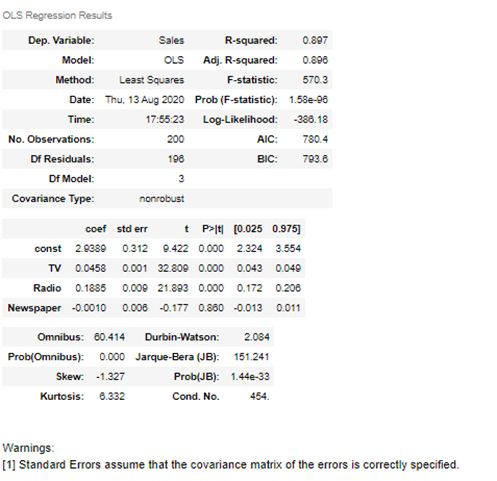
Over all our model is performing well with 89% accuracy. Let’s quickly jump in and start with the top left section first:
总体而言,我们的模型以89%的精度表现良好。 让我们快速进入并首先从左上方开始:
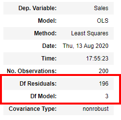
Top left section 左上方This section gives us the basic details of the model which you can read and understand like which is our y variable, when the model was built and so on. Lets look at the elements highlighted in red Df Residuals and Df model number here:
本节向我们提供了模型的基本详细信息,您可以阅读和理解该模型,例如哪个是我们的y变量,何时构建模型等等。 让我们在这里查看红色Df残渣和Df型号中突出显示的元素:
Df Residuals: Before we understand this term lets understand what is Df and Residuals:
Df残渣:在我们理解此术语之前,请先了解什么是Df和残渣:
Df here is Degrees of Freedom (DF) which indicates the number of independent values that can vary in an analysis without breaking any constraints.
这里的Df是自由度(DF),它表示可以在不破坏任何约束的情况下进行分析的独立值的数量。
Residuals in regression is simply the error rate which is not explained by the model. It’s the distance between the data point and the regression line.
回归中的残差只是错误率,模型未解释。 它是数据点与回归线之间的距离。
Residuals = (Observed value) — (Fitted/ Expected value)
残差=(观察值)-(拟合值/期望值)
The df (Residual) is the sample size minus the number of parameters being estimated, so it becomes df(Residual) = n — (k+1) or df(Residual) = n -k -1.
df(残差)是样本大小减去估计参数的数量,因此它变为df(残差)= n —(k + 1)或df(残差)= n -k -1。
Hence the calculation in our case is:
因此,在我们的案例中,计算为:
200 (total records)-3(number of X variables) -1 (for Degree of Freedom)
200(总记录)-3(X变量数)-1(对于自由度)
Df Model: Its simple the number of X variables in the data barring the Constant variable which is 3.
Df模型:它很简单,数据中X变量的数量不包括Constant变量3。
SECTION 2:
第2部分:
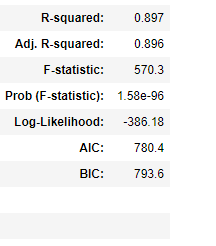
Top right section 右上方R-squared: It’s the degree of the variation in the dependent variable y that is explained by the dependent variables in X. Like in our case we can say that with the given X variables and a multi linear model, 89.7% variance is explained by the model. In regression, it also means that our predicted values are 89.7% closer to the actual value i.e y. R2 and attain values between 0 to 1.
R平方: X中的因变量解释的是因变量y的变化程度。就像我们的情况,我们可以说,在给定的X变量和多重线性模型的情况下,可以解释为89.7%的方差该模型。 在回归中,这也意味着我们的预测值与实际值y接近89.7%。 R2的值在0到1之间。
The drawback with an R2 score it that, more the number of variables in X, R2 has a tendency to be constant or increase even by a miniscule number. However, the new added variable may or may not be significant.
R2的缺点是,X中的变量数量更多,R2趋于恒定或增加甚至很小的数字。 但是,新添加的变量可能会或可能不会很重要。
R2 = Variance Explained by the model / Total Variance
R2 =方差由模型解释/总方差
OLS Model: Overall model R2 is 89.7%
OLS模型:总体模型R2为89.7%
Adjusted R-squared: This resolves the drawback of R2 score and hence is known to be more reliable. Adj. R2 doesn’t consider the variables which are not significant for the model. In a single linear regression, the value of R2 and Adjusted R2 will be the same. If more number of insignificant variables are added to the model, the gap between R2 and Adjusted R2 will keep increasing.
调整后的R平方:解决了R2分数的缺点,因此已知更为可靠。 调整 R2不考虑对模型不重要的变量。 在单个线性回归中,R2和调整后R2的值将相同。 如果将更多无关紧要的变量添加到模型中,则R2和调整后的R2之间的差距将不断增大。
Adjusted R Squared = 1 — [((1 — R2) * (n — 1)) / (n — k — 1)]
调整后的R平方= 1-[(((R-R2)*(n-1))/(n-k-1)]
Where n — number of records and k is number of significant variables barring constant.
其中n-记录数,k是不包含常数的有效变量数。
OLS Model: Adjusted R2 for the model is 89.6% which is 0.1% less than R2.
OLS模型:模型的调整后R2为89.6%,比R2小0.1%。
F-statistic and Prob(F-statistic): Here ANOVA is applied on the model with the following hypothesis:
F统计量和Prob(F统计量):此处将ANOVA用于以下假设的模型:
H0: b1, b2, b3 (Regression coefficients) are 0 or model with no independent variables fits the data better.
H0: b1,b2,b3(回归系数)为0或没有自变量的模型更适合数据。
H1: Atleast 1 of the coefficients (b1,b2,b3) is not equal to 0 or the current model with independent variable fits the data better than the intercept only model.
H1:系数(b1,b2,b3)的至少1个不等于0,或者具有自变量的当前模型比仅截距模型更适合数据。
Now practically speaking, having all of the independent variables to have coefficients 0 is not likely and we end up Rejecting the null hypothesis. However, it’s possible that each variable isn’t predictive enough on its own to be statistically significant. In other words, your sample provides sufficient evidence to conclude that your model is significant, but not enough to conclude that any individual variable is significant.
现在实际上,使所有自变量的系数都为0的可能性不大,我们最终拒绝了原假设。 但是,可能每个变量本身的预测性不足以具有统计意义。 换句话说,您的样本提供了足够的证据来推断您的模型很重要,但是不足以得出任何单个变量都有意义的结论。
F-statistic = Explained variance / unexplained variance
F统计=解释方差/无法解释方差
OLS Model: The F-stat probability is 1.58e-96 which is much lower than 0.05 which is or alpha value. It simply means that the probability of getting atleast 1 coefficient to be a nonzero value is 1.58e-96.
OLS模型: F-stat概率为1.58e-96,远低于或alpha值0.05。 这仅表示将至少1个系数设为非零值的可能性为1.58e-96。
Log-Likelihood: Log Likelihood value is a measure of goodness of fit for any model or to derive the maximum likelihood estimator. Higher the value, better is the model. We should remember that Log Likelihood can lie between -Inf to +Inf. Hence, the absolute look at the value cannot give any indication. The estimator is obtained by solving that is, by finding the parameter that maximizes the log-likelihood of the observed sample .
对数似然:对数似然值是对任何模型的拟合优度的度量,或者是得出最大似然估计值的度量。 价值越高,模型越好。 我们应该记住,对数似然可以位于-Inf到+ Inf之间。 因此,该值的绝对值不能给出任何指示。 通过求解,即通过找到使观察到的样本的对数似然性最大化的参数来获得估计量。
AIC and BIC: Akaike Information Criterion(AIC) and Bayesian Information Criterion (BIC) are 2 methods of scoring and selecting model.
AIC和BIC: Akaike信息标准(AIC)和贝叶斯信息标准(BIC)是评分和选择模型的两种方法。
AIC = -2/N * LL + 2 * k/N
AIC = -2 / N * LL + 2 * k / N
BIC = -2 * LL + log(N) * k
BIC = -2 * LL + log(N)* k
Where N is the number of examples in the training dataset, LL is the log-likelihood of the model on the training dataset, and k is the number of parameters in the model.
其中N是训练数据集中的样本数,LL是训练数据集中模型的对数似然性,k是模型中参数的数目。
The score, as defined above, is minimized, e.g. the model with the lowest AIC and BIC is selected.
如上定义的分数被最小化,例如,选择具有最低AIC和BIC的模型。
The quantity calculated is different from AIC, although can be shown to be proportional to the AIC. Unlike the AIC, the BIC penalizes the model more for its complexity, meaning that more complex models will have a worse (larger) score and will, in turn, be less likely to be selected.
尽管可以显示与AIC成比例,但计算的数量与AIC不同。 与AIC不同,BIC对其模型的复杂性加重了惩罚,这意味着更复杂的模型将具有较差的(较大的)分数,从而选择的可能性也较小。
SECTION 3:
第3部分:
Woof.. that was a lot of information. We have 2 more sections to go, Lets jump into the central part which is the main part of the summary:
Woof ..那是很多信息。 我们还有2个部分,让我们跳到中央部分,这是摘要的主要部分:
Central section 中央部分Now we know, the column coef is the value of b0, b1, b2 and b3. So the equation of the line is:
现在我们知道,列系数是b0,b1,b2和b3的值。 所以这条线的等式是:
y = 2.94 + 0.046 * (TV) + 0.188* (Radio) + (-0.001)*(Newspaper)
y = 2.94 + 0.046 *(电视)+ 0.188 *(广播)+(-0.001)*(报纸)
Std err is the standard error for each variable, it’s the distance that the variable is away from the regression line.
Std err是每个变量的标准误差,它是变量距回归线的距离。
t and P>|t|: t is simply the t-stat value of each variable with the following hypothesis:
t和P> | t |:t只是每个变量的t-stat值,其假设如下:
H0: Slope / Coefficient = 0
H0:斜率/系数= 0
H1: Slope / Coefficient is not = 0
H1:斜率/系数不等于0
Basis this, it gives us the t stat values and the P>|t| gives us the p-value. With alpha at 5%, we measure if the variables are significant.
基于此,它给出了t stat值和P> | t |。 给我们p值。 在5%的alpha值下,我们测量变量是否显着。
[0.025, 0.975] — At default 5% alpha or 95% Confidence interval, if the coef value lies in this region, we say that the coef value lies within the Acceptance region.
[0.025,0.975] -在默认的5%alpha或95%置信区间下,如果coef值位于此区域内,则表示该coef值位于“接受”区域内。
Looking at the p-values, we know we have to remove ‘Newspaper’ from our list and it’s not a significant variable. Before we come to that lets quickly interpret the last section of the model.
查看p值,我们知道我们必须从列表中删除“报纸”,这不是一个重要的变量。 在开始之前,让我们快速解释一下模型的最后一部分。
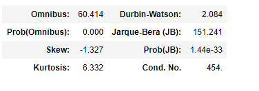
SECTION 4:
第4节:
Botton section 博顿区Omnibus: They test whether the explained variance in a set of data is significantly greater than the unexplained variance, overall. Its a test of the skewness and kurtosis of the residual. We hope for the Omnibus score to be close to 0 and its probability close to 1 which means the residuals follow normalcy.
综合:他们测试了一组数据中的解释方差是否总体上大于无法解释的方差。 它是对残留量的偏度和峰度的测试。 我们希望Omnibus分数接近0,概率接近1,这意味着残差遵循常态。
In our case Omnibus score is very high, way over 60 and its probability is 0. This means our residuals or error rate does not follow a normal distribution.
在我们的案例中,Omnibus得分非常高,超过60,其概率为0。这意味着我们的残差或错误率未遵循正态分布。
Skew — Its a measure of data symmetry. We want to see something close to zero, indicating the residual distribution is normal. Note that this value also drives the Omnibus.
倾斜-其 数据对称性的度量。 我们希望看到接近零的值,这表明残差分布是正态的。 注意,该值也驱动综合总线。
We can see that our residuals are negatively skewed at -1.37.
我们可以看到我们的残差在-1.37处负偏斜。
Kurtosis — Its a measure of curvature of the data. Higher peaks lead to greater Kurtosis. Greater Kurtosis can be interpreted as a tighter clustering of residuals around zero, implying a better model with few outliers.
峰度-它是数据曲率的度量。 更高的峰导致更大的峰度。 峰度较大可以解释为零附近的残差更紧密的聚类,这意味着具有较少异常值的更好模型。
Looking at the results, our kurtosis is 6.33 which means our data doesn’t have outliers.
从结果看,我们的峰度为6.33,这意味着我们的数据没有异常值。
Durbin-Watson — The Durbin Watson (DW) statistic is a test for autocorrelation in the residuals from a statistical regression analysis. The Durbin-Watson statistic will always have a value between 0 and 4. A value of 2.0 means that there is no autocorrelation detected in the sample.
Durbin-Watson- Durbin Watson(DW)统计量是对统计回归分析中残差自相关的检验。 Durbin-Watson统计信息将始终具有介于0和4之间的值。值为2.0表示在样本中未检测到自相关。
Durbin-Watson value is 2.084 which is very close to 2 and we conclude that the data doesn’t have autocorrelation.
Durbin-Watson值为2.084,非常接近2,我们得出的结论是数据不具有自相关。
Note: Autocorrelation, also known as serial correlation, it is the similarity between observations as a function of the time lag between them.
注意:自相关,也称为序列相关,它是观测值之间的相似度,是它们之间时间滞后的函数。
Jarque-Bera (JB)/Prob(JB) — JB score simply tests the normality of the residuals with the following hypothesis:
Jarque-Bera(JB)/ Prob(JB)— JB分数仅使用以下假设测试残差的正态性:
H0: Residuals follow a normal distribution
H0:残差服从正态分布
H1: Residuals don’t follow a normal distribution
H1:残差不服从正态分布
Prob(JB) is very low, close to 0 and hence we reject the null hypothesis.
Prob(JB)非常低,接近于0,因此我们拒绝原假设。
Cond. No. : The condition number is used to help diagnose collinearity. Collinearity is when one independent variable is close to being a linear combination of a set of other variables.
条件。 编号:条件编号用于帮助诊断共线性。 共线性是当一个自变量接近于一组其他变量的线性组合时。
The condition number is 454 in our case, when we reduce our variables lets see how the score reduces.
在我们的例子中,条件数是454,当我们减少变量时,让我们看看分数如何减小。
Okay we are almost at the end of our article, we have already seen the interpretation of each and every element in this OLS model. Just 1 last section where we update our OLS model and compare the results:
好的,我们快到本文结尾了,我们已经看到了此OLS模型中每个元素的解释。 仅在最后一节中,我们更新了我们的OLS模型并比较了结果:
If we look at our model, only Newspaper with p-value 0.86 is higher than 0.05. Hence we will rebuild a model after removing the Newspaper:
如果看我们的模型,只有p值为0.86的报纸高于0.05。 因此,我们将在删除报纸后重建模型:
Updated OLS model (removed Newspaper) 更新了OLS模型(已删除报纸)Please note as already mentioned, the coefficient values for each variable is dependent on the other. Hence we should always remove columns 1 by 1 so that we can gauge the difference.
如前所述, 请注意 ,每个变量的系数值都依赖于另一个。 因此,我们应始终删除第1列到第1列,以便我们可以衡量差异。
When we remove the newspaper, our accuracy levels do not change however the coefficients have been updated. However the AIC, BIC scores and Cond. No. have reduced which proves we have improved the efficiency of the model.
当我们取出报纸时,我们的准确度不会改变,但是系数已经更新。 但是AIC,BIC得分和Cond。 数量减少了,这证明我们提高了模型的效率。
Wow! we are finally at the end of this article. There are lots of elements in an OLS model which we have interpreted above. I have tried to simplify and throw light on each and every section of the OLS summary.
哇! 我们终于到了本文的结尾。 上面我们已经解释了,OLS模型中有很多元素。 我已经尝试简化并简要介绍OLS摘要的每个部分。
If you have any queries do ask in the comments also if you find something amiss do let me know.
如果您有任何疑问,请在评论中询问是否还有不对劲,请告诉我。
Drop in a clap if you learnt something new in this article.
如果您学到了本文的新内容,请稍加鼓掌。
翻译自: https://medium.com/analytics-vidhya/ordinary-least-squared-ols-regression-90942a2fdad5
