python-opencv
python-opencv
文章目录
- python-opencv
- 前言
- 一、图像处理
-
- 1.二值化
-
- threshold
- 2.图像平滑
-
- 均值滤波 blur
- 方框滤波 boxFilter
- 高斯滤波 GaussianBlur
- 中值滤波 median
- 3.形态学
-
- 膨胀 dilate
- 腐蚀 erode
- 开运算 MORPH_OPEN
- 闭运算 MORPH_CLOSE
- 梯度运算 MORPH_GRADIENT
- 礼帽 MORPH_TOPHAT
- 黑帽 MORPH_BLACKHAT
- 4.图像梯度 -- 获得边缘轮廓
-
- Sobel 算子
- Scharr 算子
- laplacian 算子
- Canny 边缘检测
- 5.图像金字塔
-
- 高斯金字塔
- 拉普拉斯金字塔
- 6.图像轮廓
- 7.模板匹配
- 8.直方图
- 9.傅里叶变换
- 10. 实战
-
- 一、 银行卡号识别
- 二、 文档扫描OCR识别
- 二、图像特征
-
- 1. harris 角点检测
- 2. sift
- 3.特征匹配
- 4.图像拼接
- 总结
前言
文章为opencv笔记
一、图像处理
1.二值化
threshold
ret,threshold_img=cv2.threshold(img,80,255,cv2.THRESH_BINARY)
cv2.imshow('threshold',threshold_img)
2.图像平滑
均值滤波 blur,方框滤波 boxFilter
高斯滤波 GaussianBlur, 中值滤波 median
均值滤波 blur
方框滤波 boxFilter
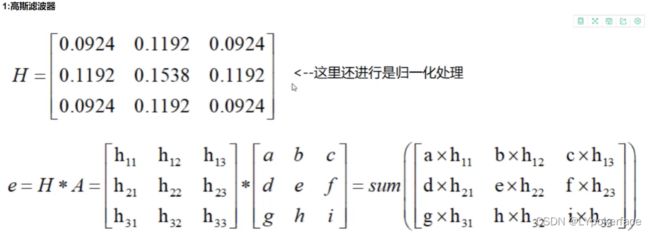
高斯滤波 GaussianBlur
中值滤波 median
#均值滤波
#[1,1,1
# 1,1,1
# 1,1,1]
blur=cv2.blur(img,(3,3))
cv2.imshow('blur',blur)

#方框滤波,基本和均值一样,可以选择归一化
box=cv2.boxFilter(img,-1,(3,3),normalize=True)

#高斯滤波,高斯模糊的卷积核里的数值是满足高斯分布,相当于更重视中间的
#[0.6,0.8,0.6
# 0.8,1,0.8
# 0.6,0.8,0.6]
guass=cv2.GaussianBlur(img,(5,5),1)

#中值滤波 - 相当于用中值代替
median=cv2.medianBlur(img,5)

#展示所有
res=np.hstack((blur,guass,median))
print(res)
cv2.imshow('res',res)
3.形态学
膨胀 dilate
膨胀 : 相当于最大值滤波,用矩阵中最大值替换中心元素,扩大白色区域
腐蚀 erode
腐蚀:相当于最小值滤波。最小值替换中心像素,扩大黑色区域
#numpy定义核大小,并标记为灰度格式
kernel=np.ones((3,3),np.uint8)

#核的大小和形状
kernel=cv2.getStructuringElement(cv2.MORPH_RECT,(5,5))
#执行3次腐蚀操作
erode=cv2.erode(threshold_img,kernel,iterations=3)
#执行4次膨胀操作
dilate=cv2.dilate(threshold_img,kernel,iterations=4)
开运算 MORPH_OPEN
开运算:先腐蚀,后膨胀
闭运算 MORPH_CLOSE
闭运算:先膨胀,后腐蚀
open_img=cv2.morphologyEx(img,cv2.MORPH_OPEN,kernel)
close_img=cv2.morphologyEx(img,cv2.MORPH_CLOSE,kernel)
梯度运算 MORPH_GRADIENT
梯度运算:梯度=膨胀-腐蚀
gradient=cv2.morphologyEx(img,cv2.MORPH_GRADIENT,kernel)
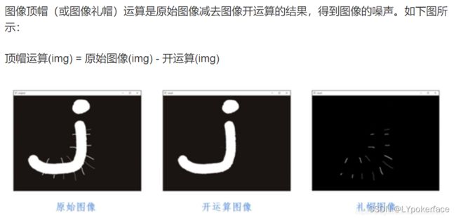
礼帽 MORPH_TOPHAT
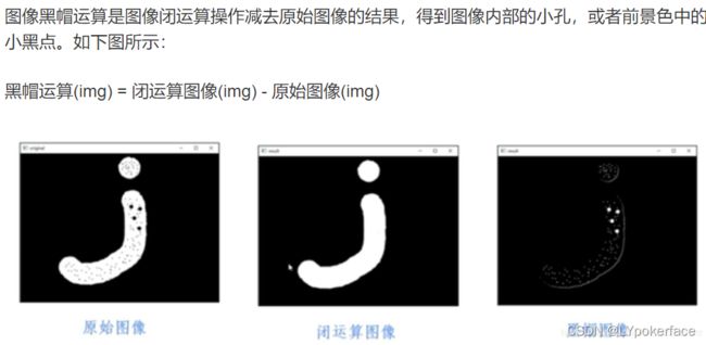
黑帽 MORPH_BLACKHAT
礼帽 与 黑帽
礼帽=原始输入-开运算结果(得到图像噪声)
黑帽=闭运算-原始输入(得到图像内部的小孔,或前景色中的小黑点)
tophat=cv2.morphologyEx(img,cv2.MORPH_TOPHAT,kernel)
blackhat=cv2.morphologyEx(img,cv2.MORPH_BLACKHAT,kernel)
4.图像梯度 – 获得边缘轮廓

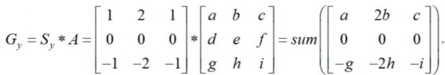
Sobel 算子
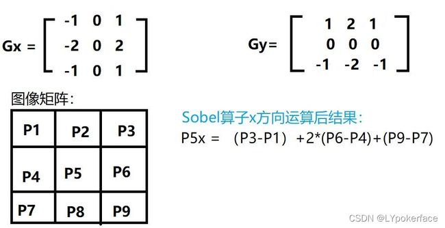
sobel_x=cv2.Sobel(img,cv2.CV_64F,1,0,ksize=3)
#sobel算子运算后,会出现负值,负值取绝对值,结果最大值为255,范围0-255
sobel_x=cv2.convertScaleAbs(sobel_x)

sobel_y=cv2.Sobel(img,cv2.CV_64F,0,1,ksize=3)
sobel_y=cv2.convertScaleAbs(sobel_y)
#建议分开取 x,y再结合,直接sobel同时求x,y方向图像会有些边缘点结果不同
sobel_xy=cv2.addWeighted(sobel_x,0.5,sobel_y,0.5,0)
cv2.imshow("sobel_img",sobel_xy)
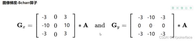
Scharr 算子
scharrx=cv2.Scharr(img,cv2.CV_64F,1,0,ksize=3)
scharrx=cv2.convertScaleAbs(scharrx)
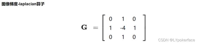
laplacian 算子
laplacian=cv2.Laplacian(img,cv2.CV_64F)
laplacian=cv2.convertScaleAbs(laplacian)
从左-右,依次是sobel – scharr – laplacian ,处理后的不同边缘效果
Canny 边缘检测
(1)使用高斯滤波器,以平滑图像,滤除噪声
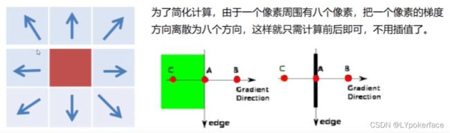
(2)计算图像中每个像素点的梯度强度和方向
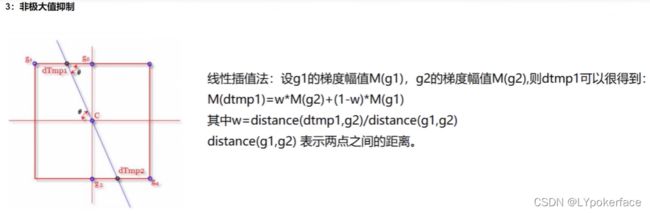
(3)应用非极大值抑制,以消除边缘检测带来的杂散响应
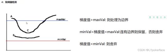
(4)应用双阈值检测来确定真实的和潜在的边缘
(5)通过抑制孤立的弱边缘最终完成边缘检测

c1=cv2.Canny(img,80,150)
5.图像金字塔
高斯金字塔
向下采样法(缩小)
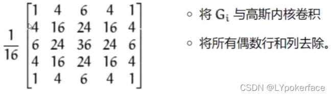
down=cv2.pyrDown(img)
向上采样法(放大)
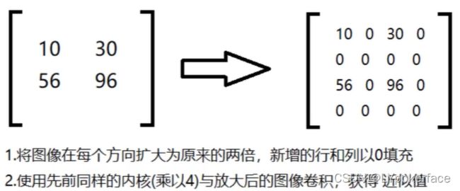
up=cv2.pyrUp(img)
拉普拉斯金字塔
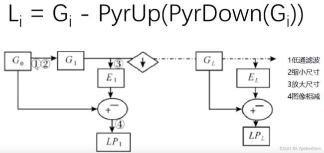
#拉普拉斯金字塔
l_down=cv2.pyrDown(img)
l_down_up=cv2.pyrUp(down)
l_l=img-l_down_up
cv2.imshow('l_l',l_l)
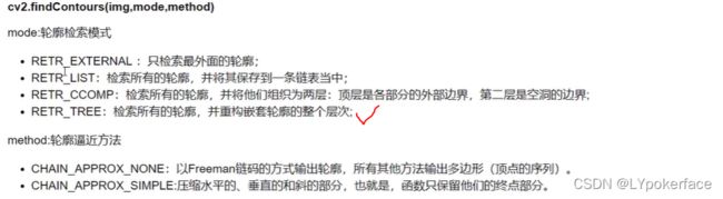
6.图像轮廓
img=cv2.imread('11.png')
gray=cv2.cvtColor(img,cv2.COLOR_BGR2GRAY)
ret,thresh=cv2.threshold(gray,127,255,cv2.THRESH_BINARY)
cv2.imshow('thresh',thresh)

contours, hierarchy=cv2.findContours(thresh,cv2.RETR_TREE,cv2.CHAIN_APPROX_NONE)

#传入绘制图像,轮廓,轮廓索引,颜色模式,线条厚度
#注意需要copy,避免修改原图像
draw_img=img.copy()
res=cv2.drawContours(draw_img,contours,5,(0,0,255),2)
cv2.imshow('res',res)

#轮廓特征
cnt=contours[0]
area=cv2.contourArea(cnt)#面积
arc=cv2.arcLength(cnt,True)#周长

#轮廓近似
epsilon=0.1*cv2.arcLength(cnt,True)
approx=cv2.approxPolyDP(cnt,epsilon,True)

#边界矩形
x,y,w,h=cv2.boundingRect(cnt)
img_rect=cv2.rectangle(img,(x,y),(x+w,y+h),(0,255,0),2)
cv2.imshow('img_rect',img_rect)

#外接圆
(x,y),radius=cv2.minEnclosingCircle(cnt)
center=(int(x),int(y))
radius=int(radius)
img=cv2.circle(img,center,radius,(255,0,0),2)
cv2.imshow('img',img)
7.模板匹配
模板匹配和卷积原理很像,模板在原图像上从原点开始滑动,计算模板与(图像被模板覆盖的地方)的差别程度,这个差别程度的计算方法在opencv里有6种,然后将每次计算的结果放入一个矩阵里,作为结果输出。
常用匹配方式为 带归一化的方式比较准确

import cv2
import numpy as np
import matplotlib.pyplot as plt

img=cv2.imread('1.jpg')
template=cv2.imread('2.JPG')

h,w=template.shape[:2]
print(img.shape)
print(template.shape)

res=cv2.matchTemplate(img,template,cv2.TM_CCOEFF_NORMED)
print(res.shape)
min_val,max_val,min_loc,max_loc=cv2.minMaxLoc(res)

threshold=0.8
#取匹配程度大于80的坐标
loc=np.where(res>=threshold)
for pt in zip(*loc[::-1]):
    bottom_right=(pt[0]+w,pt[1]+h)
    cv2.rectangle(img,pt,bottom_right,(0,0,255),1)
cv2.imshow('match',img)
cv2.waitKey(0)
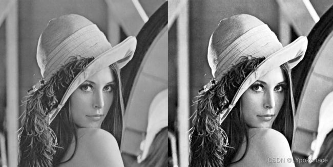
8.直方图

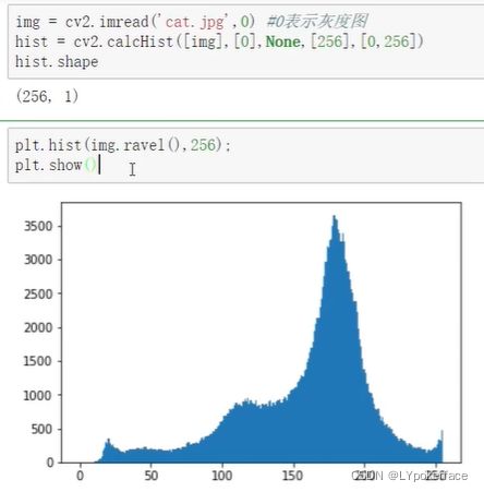
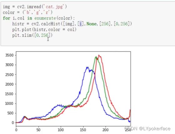
img_hist=cv2.imread('1.jpg',0)
hist=cv2.calcHist([img_hist],[0],None,[256],[0,256])
#plt.hist(img_hist.ravel(),256)
#plt.show()

#直方图均衡化
equ=cv2.equalizeHist(img_hist)
ress=np.hstack((img_hist,equ))
cv2.imshow('1',ress)
(右图)均衡化后:
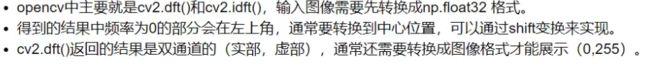
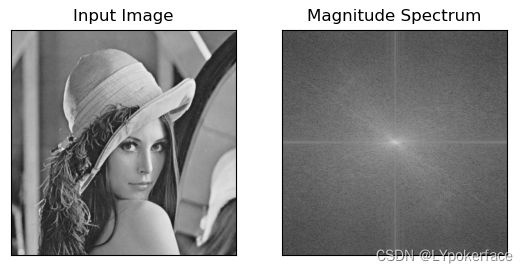
9.傅里叶变换
傅里叶变换的作用:
》高频:变化剧烈的灰度分量,例如边界
》低频:变化缓慢的灰度分类,例如一片大海
滤波:
》低通滤波器:只保留低频,会使图像模糊
》高通滤波器:只保留高频,会使图像细节增强
img=cv2.imread('1.jpg',0)
img_float32=np.float32(img)

dft=cv2.dft(img_float32,flags=cv2.DFT_COMPLEX_OUTPUT)
dft_shift=np.fft.fftshift(dft)

#得到灰度图能表示的形式
magnitude_spectrum=20*np.log(cv2.magnitude(dft_shift[:,:,0],dft_shift[:,:,1]))

plt.subplot(121),plt.imshow(img,cmap='gray')
plt.title('Input Image'),plt.xticks([]),plt.yticks([])
plt.subplot(122),plt.imshow(magnitude_spectrum,cmap='gray')
plt.title('Magnitude Spectrum'),plt.xticks([]),plt.yticks([])
plt.show()

#中心位置
rows,cols=img.shape
crow,ccol=int(rows/2),int(cols/2)

#滤波
# 1-低通滤波     2-高通滤波
flag=[1,0]

for i in flag:

	mask=np.zeros((rows,cols,2),np.uint8)
	mask[crow-30:crow+30,ccol-30:ccol+30]=i

	#IDFT
	f_shift=dft_shift*mask
	f_ishift=np.fft.ifftshift(f_shift)
	img_back=cv2.idft(f_ishift)
	img_back=cv2.magnitude(img_back[:,:,0],img_back[:,:,1])

	plt.subplot(121),plt.imshow(img,cmap='gray')
	plt.title('Input Image'),plt.xticks([]),plt.yticks([])
	plt.subplot(122),plt.imshow(img_back,cmap='gray')
	plt.title('Result'),plt.xticks([]),plt.yticks([])
	plt.show()

10. 实战
一、 银行卡号识别


import cv2
import matplotlib.pyplot as plt
import numpy as np

#显示
def imShow(img,name='img'):
	cv2.imshow(name,img)
	cv2.waitKey(0)

# 轮廓排序
def sort_contours(cnts, method="left-to-right"):
	reverse = False
	i = 0

	if method == 'left-to-right' or method == 'right-to-left':
		if method == 'right-to-left':
			reverse = True
	if method == 'bottom-to-top' or method == 'top-to-bottom':
		i = 1
		if method == 'bottom-to-top':
			reverse = True
	boundingBoxes = [cv2.boundingRect(c) for c in cnts]
	(cnt, boundingBoxes) = zip(*sorted(zip(cnts, boundingBoxes), key=lambda b: b[1][i], reverse=reverse))
	return cnt, boundingBoxes

#resize
def myResize(img,row):
	r,c,n=img.shape
	col=c/r*row
	return cv2.resize(img,(int(col),int(row)))

# 读模板
img_template_0 = cv2.imread('card/number.png')
img_template = cv2.cvtColor(img_template_0, cv2.COLOR_BGR2GRAY)
# 二值化
ref = cv2.threshold(img_template, 10, 255, cv2.THRESH_BINARY_INV)[1]
#imShow(ref)
# 找轮廓
contours, hierarchy = cv2.findContours(ref.copy(), cv2.RETR_EXTERNAL, cv2.CHAIN_APPROX_NONE)
cv2.drawContours(img_template_0, contours, -1, (0, 0, 255), 3)
#imShow(img_template_0,'template')

refCnts = sort_contours(contours, method='left-to-right')[0]
digits = {}

# 遍历每一个轮廓
for (i, c) in enumerate(refCnts):
	# 计算外接矩形并且resize成合适大小
	(x, y, w, h) = cv2.boundingRect(c)
	roi = ref[y:y + h, x:x + w]
	roi = cv2.resize(roi, (57, 88))
	# 每一个数字对应每一个模板
	digits[i] = roi

#初始化卷积核
rectKernel=cv2.getStructuringElement(cv2.MORPH_RECT,(20,1))
sqKernel=cv2.getStructuringElement(cv2.MORPH_RECT,(5,5))

#读取输入图像,预处理
img = cv2.imread('card/3.png')
img=myResize(img,300)
gray=cv2.cvtColor(img,cv2.COLOR_BGR2GRAY)
#imShow(img,'orc')

#顶帽操作,突出更明亮的区域
tophat=cv2.morphologyEx(gray,cv2.MORPH_TOPHAT,rectKernel)
#imShow(tophat,'tophat')

#sobel轮廓
gradx=cv2.Sobel(tophat,cv2.CV_32F,1,0,-1)

gradx=np.absolute(gradx)
(minval,maxval)=(np.min(gradx),np.max(gradx))
gradx=(255*((gradx-minval)/(maxval-minval)))
gradx=gradx.astype('uint8')

gradx=cv2.morphologyEx(gradx,cv2.MORPH_CLOSE,rectKernel)
ret,con=cv2.threshold(gradx,0,255,cv2.THRESH_BINARY|cv2.THRESH_OTSU)
gradx=cv2.morphologyEx(con,cv2.MORPH_CLOSE,rectKernel)
#imShow(gradx,'gradx')

con,hie=cv2.findContours(gradx.copy(), cv2.RETR_EXTERNAL, cv2.CHAIN_APPROX_NONE)
#cv2.drawContours(img, con, -1, (0, 0, 255), 3)
#imShow(img,'draw')

loc=[]
for (i,c) in enumerate(con):
	(x,y,w,h)=cv2.boundingRect(c)
	ar=w/float(h)

	if ar>2.5 and ar<4.0:
		if(w>50 and w<100)and (h>15 and h<30):
			loc.append((x,y,w,h))
#符合的轮廓排序
loc=sorted(loc,key=lambda x:x[0])

print('轮廓数量:'+str(len(loc)))

output=[]

for (i,(gx,gy,gw,gh))in enumerate(loc):
	groupOutput=[]

	#根据坐标提取每一个组
	group=gray[gy-5:gy+gh+5,gx-5:gx+gw+5]
	#预处理
	group=cv2.threshold(group,0,255,cv2.THRESH_BINARY|cv2.THRESH_OTSU)[1]
	#imShow(group,'group')
	#找到每一组的轮廓
	con,hie=cv2.findContours(group.copy(),cv2.RETR_EXTERNAL,cv2.CHAIN_APPROX_NONE)
	con=sort_contours(con,'left-to-right')[0]

	#计算每一组中的每一个数值
	for c in con:
		(x,y,w,h)=cv2.boundingRect(c)
		roi=group[y:y+h,x:x+w]
		roi=cv2.resize(roi,(57,88))
		#imShow(roi,'roi')

		#计算匹配得分
		scores=[]
		#在模板中计算每一个得分
		for(digit,digitsROI) in digits.items():
			result=cv2.matchTemplate(roi,digitsROI,cv2.TM_CCOEFF)
			score=cv2.minMaxLoc(result)[1]
			scores.append(score)
		#得到最合适的数字
		groupOutput.append(str(np.argmax(scores)))

	#画出来
	cv2.rectangle(img,(gx-5,gy-5),(gx+gw+5,gy+gh+5),(0,0,255),1)
	cv2.putText(img,''.join(groupOutput),(gx,gy-15),cv2.FONT_HERSHEY_SIMPLEX,0.65,(0,255,0),1)

	output.extend(groupOutput)
print(str(output))

imShow(img,'OCR')
cv2.waitKey(0)
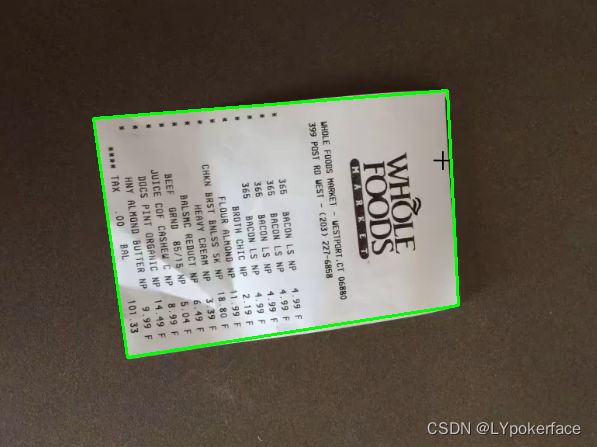
二、 文档扫描OCR识别
识别OCR部分,我们会简单点用到tesseract来识别,附上下载地址,先下载然本地exe识别软件,后再python IDE里pip install pytesseract安装包即可,pytesseract.py文件会调用本地的exe进行识别OCR:
tesseract的下载地址:https://digi.bib.uni-mannheim.de/tesseract/
pip install pytesseract安装后,需要修改py文件的路径为安装的路径,并需要把路径加入系统变量。

import cv2
import numpy as np
from scipy.spatial import distance as dist
import os
import pytesseract
# 显示
def imShow(img, name='img'):
cv2.imshow(name, img)
#cv2.waitKey(0)
def order_points(pts):
# sort the points based on their x-coordinates
xSorted = pts[np.argsort(pts[:, 0]), :]
# grab the left-most and right-most points from the sorted
# x-roodinate points
leftMost = xSorted[:2, :]
rightMost = xSorted[2:, :]
# now, sort the left-most coordinates according to their
# y-coordinates so we can grab the top-left and bottom-left
# points, respectively
leftMost = leftMost[np.argsort(leftMost[:, 1]), :]
(tl, bl) = leftMost
# now that we have the top-left coordinate, use it as an
# anchor to calculate the Euclidean distance between the
# top-left and right-most points; by the Pythagorean
# theorem, the point with the largest distance will be
# our bottom-right point
D = dist.cdist(tl[np.newaxis], rightMost, "euclidean")[0]
(br, tr) = rightMost[np.argsort(D)[::-1], :]
# return the coordinates in top-left, top-right,
# bottom-right, and bottom-left order
return np.array([tl, tr, br, bl], dtype="float32")
def four_point_transform(image, pts):
rect=order_points(pts)
(tl,tr,br,bl)=rect
#计算输入的w和h值
widthA=np.sqrt(((br[0]-bl[0])**2)+((br[1]-bl[1])**2))
widthB=np.sqrt(((tr[0]-tl[0])**2)+((tr[1]-tl[1])**2))
maxWidth=max(int(widthA),int(widthB))
heightA = np.sqrt(((br[0] - tr[0]) ** 2) + ((br[1] - tr[1]) ** 2))
heightB = np.sqrt(((bl[0] - tl[0]) ** 2 )+ ((bl[1] - tl[1]) ** 2))
maxHeight = max(int(heightA), int(heightB))
#变换后对应坐标位置
dst=np.array([
[0,0],[maxWidth-1,0],[maxWidth-1,maxHeight-1],[0,maxHeight-1]],dtype='float32')
#计算变换矩阵
M=cv2.getPerspectiveTransform(rect,dst)
warped=cv2.warpPerspective(image,M,(maxWidth,maxHeight))
#返回变换后的结果
return warped
img = cv2.imread('card/file3.png')
ratio = img.shape[0] / 500.0
orig = img.copy()
r, c, n = img.shape
image = cv2.resize(orig, (int(c / ratio), 500))
# 预处理
gray = cv2.cvtColor(image, cv2.COLOR_BGR2GRAY)
gray = cv2.GaussianBlur(gray, (5, 5), 0)
edged = cv2.Canny(gray, 75, 200)
print('STEP 1 : 边缘检测')
imShow(edged, 'edged')
# 轮廓检测
cnts = cv2.findContours(edged.copy(), cv2.RETR_LIST, cv2.CHAIN_APPROX_SIMPLE)[0]
cnts = sorted(cnts, key=cv2.contourArea, reverse=True)[:5]
# 遍历轮廓
for c in cnts:
peri = cv2.arcLength(c, True)
# 近似拟合一个封闭轮廓
approx = cv2.approxPolyDP(c, 0.02 * peri, True)
if len(approx) == 4:
screenCnt = approx
break
print('STEP 2 : 获取轮廓')
cv2.drawContours(image, [screenCnt], -1, (0, 255, 0), 2)
imShow(image, 'OutLine')
out=four_point_transform(img,screenCnt.reshape(4,2)*ratio)
imShow(out,'out')
print('STEP 3 : 透视变换')
#保存转换后的图片
save_img=cv2.cvtColor(out,cv2.COLOR_BGR2GRAY)
ret,save_img=cv2.threshold(save_img,0,255,cv2.THRESH_BINARY|cv2.THRESH_OTSU)
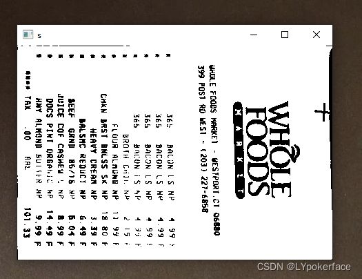
imShow(save_img,'s')
cv2.imwrite('123.jpg',save_img)
#用pytesseract识别OCR
import pytesseract
from PIL import Image
a=Image.open('123.jpg')
test=pytesseract.image_to_string(a)
print(test)
cv2.waitKey(0)
二、图像特征
这部分原理比较难,好好看文章视频理解吧····
1. harris 角点检测
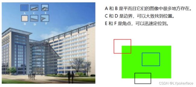
Harris 角点检测原理参考文章
import cv2
import numpy as np
import matplotlib.pyplot as plt

image=cv2.imread('calibrate.jpg')
gray=cv2.cvtColor(image,cv2.COLOR_BGR2GRAY)
#角点检测,输入图像必须是float32
gray=np.float32(gray)

dst=cv2.cornerHarris(gray,2,3,0.04)

image[dst>0.01*dst.max()]=[0,0,255]

#plt.figure(figsize=(10,8),dpi=100)
#plt.imshow(image[:,:,::-1]),plt.title('Harris 角点检测')
#plt.xticks(),plt.yticks()
#plt.show()

cv2.imshow('dst',image)
cv2.waitKey(0)
2. sift
sift原理参考文章
# SIFT函数
cv2.imshow('dst',image)
cv2.waitKey(0)
#得到特征点
sift=cv2.SIFT_create()
kp=sift.detect(gray,None)
image=cv2.drawKeypoints(gray,kp,image)
cv2.imshow('draw',image)
cv2.waitKey(0)
#计算特征
kp,des=sift.compute(gray,kp)
print(np.array(kp).shape)
3.特征匹配
匹配使用的是 cv2.BFMatcher 蛮力匹配
如果需要更快速完成操作,可以尝试使用cv2.FlannBasedMatcher
import cv2
import matplotlib.pyplot as plt

def myResize(img,row):
	r,c=img.shape[:2]
	col=c/r*row
	return cv2.resize(img,(int(col),int(row)))

#特征匹配

# Brute-Force 蛮力匹配
img1=cv2.imread('pinjie3.jpg')
img2=cv2.imread('pinjie4.jpg')

img1=myResize(img1,500)
img2=myResize(img2,500)

#cv2.imshow('img1',img1)
#cv2.imshow('img2',img2)

sift=cv2.SIFT_create()

kp1,des1=sift.detectAndCompute(img1,None)
kp2,des2=sift.detectAndCompute(img2,None)

# 蛮力匹配 -- 欧几里德距离
bf=cv2.BFMatcher(crossCheck=True)

# 1对1 的匹配
matches=bf.match(des1,des2)
matches=sorted(matches,key=lambda x:x.distance)

img3=cv2.drawMatches(img1,kp1,img2,kp2,matches[:10],None,flags=2)
cv2.imshow('1 match',img3)

# K对最佳匹配
bf=cv2.BFMatcher()

matches=bf.knnMatch(des1,des2,k=2)
good=[]
for m, n in matches:
	if m.distance<0.5*n.distance:
		good.append([m])
img4=cv2.drawMatchesKnn(img1,kp1,img2,kp2,good,None,flags=2)
cv2.imshow('K match',img4)

cv2.waitKey(0)
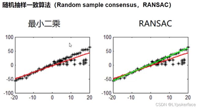
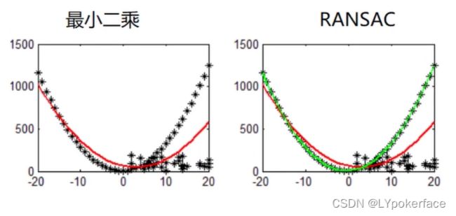
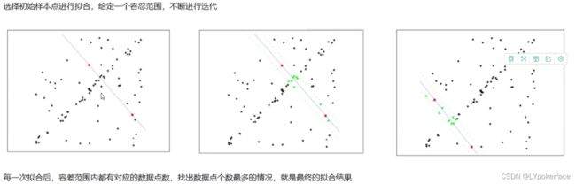
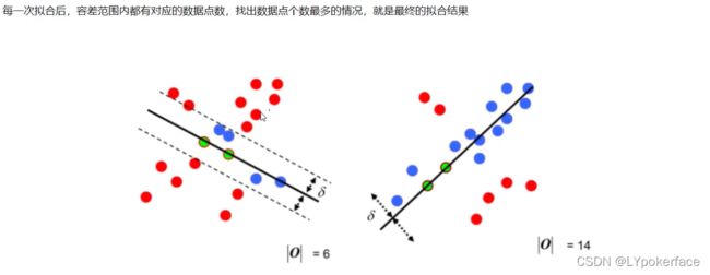
随机抽样一致性:简单描述,即是随机选择数据点拟合,限制容差范围,容差范围内数据点数最多的情况,就是最终的拟合结果。

4.图像拼接
import numpy as np
import cv2


class Stitcher:

	# 拼接函数
	def stitch(self, images, ratio=0.75, reprojThresh=4.0, showMatches=False):
		# 获取输入图片
		(imageB, imageA) = images
		# 检测A、B图片的 SIFT 关键特征点,并计算特征描述
		(kps1, features1) = self.detectAndDescribe(imageA)
		(kps2, features2) = self.detectAndDescribe(imageB)

		# 匹配两张图片的所有特征点,返回匹配结果
		M = self.matchKeypoints(kps1, kps2, features1, features2, ratio, reprojThresh)

		# 如果返回结果为空,没有匹配成功的特征点,退出算法
		if M is None:
			return None

		# 否则,提取匹配结果
		# H 是 3x3 视角变换矩阵
		(matches, H, status) = M

		# 将图片A进行视角变换
		result = cv2.warpPerspective(imageA, H, (imageA.shape[1] + imageB.shape[1], imageA.shape[0]))
		self.cv_show('result1', result)
		# 将图片B传入result图片最左端
		result[0:imageB.shape[0], 0:imageB.shape[1]] = imageB
		self.cv_show('result2', result)

		# 检测师傅显示图像匹配
		if showMatches:
			# 生成匹配图片
			vis = self.drawMatches(imageA, imageB, kps1, kps2, matches, status)
			# 返回结果
			return (result, vis)

		# 返回匹配结果
		return result

	def detectAndDescribe(self, image):
		# 将彩色图转换成灰度图
		gray = cv2.cvtColor(image, cv2.COLOR_BGR2GRAY)
		# 建立SIFT生成器
		descriptor = cv2.SIFT_create()
		# 检测SIFT特征点,并计算特征
		(kps, features) = descriptor.detectAndCompute(image, None)

		# 将结果转换成Numpy数组
		kps = np.float32([kp.pt for kp in kps])

		# 返回特征点集,及对应的描述特征
		return (kps, features)

	def matchKeypoints(self, kpsA, kpsB, featuresA, featuresB, ratio, reprojThresh):
		# 建立蛮力匹配器
		matcher = cv2.BFMatcher()

		# 使用KNN检测来自A B图的SIFT 特征匹配,K=2
		rawMatches = matcher.knnMatch(featuresA, featuresB, 2)

		matches = []
		for m in rawMatches:
			# 当最近距离 跟 次近距离的比值小于ratio值时,保留此匹配对
			if len(m) == 2 and m[0].distance < m[1].distance * ratio:
				# 存储两个点在featureA 和 featureB中的索引值
				matches.append((m[0].trainIdx, m[0].queryIdx))

		# 当筛选后的匹配对大于4时,计算视角变换矩阵
		if len(matches) > 4:
			# 获取匹配对的点坐标
			ptsA = np.float32([kpsA[i] for (_, i) in matches])
			ptsB = np.float32([kpsB[i] for (i, _) in matches])

			# 计算视角变换矩阵
			(H, status) = cv2.findHomography(ptsA, ptsB, cv2.RANSAC, reprojThresh)

			# 返回结果
			return (matches, H, status)
		return None

	def drawMatches(self, imageA, imageB, kpsA, kpsB, matches, status):
		# 初始化可视化图片,将A、B图左右连接到一起
		(hA, wA) = imageA.shape[:2]
		(hB, wB) = imageB.shape[:2]
		vis = np.zeros((max(hA, hB), wA + wB, 3), dtype="uint8")
		vis[0:hA, 0:wA] = imageA
		vis[0:hB, wA:] = imageB

		# 联合遍历,画出匹配对
		for ((trainIdx, queryIdx), s) in zip(matches, status):
			# 当点对匹配成功时,画到可视化图上
			if s == 1:
				# 画出匹配对
				ptA = (int(kpsA[queryIdx][0]), int(kpsA[queryIdx][1]))
				ptB = (int(kpsB[trainIdx][0]) + wA, int(kpsB[trainIdx][1]))
				cv2.line(vis, ptA, ptB, (0, 255, 0), 1)

		# 返回可视化结果
		return vis

	def cv_show(self, name, image):
		cv2.imshow(name, image)
		cv2.waitKey(0)

	# cv2.destroyAllWindows()

	def myResize(self, img, row):
		r, c = img.shape[0:2]
		col = c / r * row
		return cv2.resize(img, (int(col), int(row)))
import cv2
import matplotlib.pyplot as plt
import numpy as np
from Stitcher import Stitcher


imageA=cv2.imread('pinjie5.jpg')
imageB=cv2.imread('pinjie6.jpg')

#把图片拼接成全景图
stitcher=Stitcher()

imageA=stitcher.myResize(imageA,500)
imageB=stitcher.myResize(imageB,500)

(result,vis)=stitcher.stitch([imageA,imageB],showMatches=True)

cv2.imshow('Key Point Matches',vis)
cv2.imshow('Result',result)
cv2.waitKey(0)