数学杂谈：高维空间向量夹角小记

• 数学杂谈：高维空间向量夹角小记
  • 1. 问题描述
  • 2. n维空间中的均匀向量
    • 1. 2维以及3维空间中的特殊情况
      • 1. 2维空间中的均匀分布向量
      • 3. 3维空间中的均匀分布向量
    • 2. n维坐标系中的均匀向量
    • 3. 正态分布的巧妙应用
  • 3. n维空间中两向量夹角考察
  • 4. 总结 & 思考

1. 问题描述

故事起源于long long ago的时候看到的苏剑林某一篇博客当中提到了一个结论：

• 高维空间中两个随机向量大概率是相互正交的。

当时就对这个结论比较在意了，今天突然地又想到了这个问题，就想着趁着放假把这个结论验证一下。

显然，苏剑林在博客中提到的这个结论的表述是比较随意的，为了更好地定义我们的问题，我们将其细化一下：

• 对于n维中间的单位球面上的两个随机向量，他们之间的夹角$\theta$在n取大值时，趋近于90度。

要证明这个结论感觉比较难，但是要演示说明一下这个结果确实相对容易的，我们的第一反应就是蒙特卡洛模拟一下，实际生成$N$组$n$维空间上的均匀单位向量，然后考察一下他们之间的角度分布。

但是，要做到这件事，我们首先需要生成一下n维空间当中的均匀分布的单位向量。

2. n维空间中的均匀向量

1. 2维以及3维空间中的特殊情况

首先，我们来考察一些简单的情况，即2维和3维空间当中的情况。

1. 2维空间中的均匀分布向量

二维空间中的均匀分布向量其实就是单位圆上面的均匀分布向量，因此，我们只需要给出一个$0$到$\pi$之间均匀分布的角度$\varphi$即可得到一个均匀分布的单位向量$v=(sin\theta ,cos\theta )$。

3. 3维空间中的均匀分布向量

对于三维的情况，事实上我相信大部分读者只要熟悉坐标系变换的话就还是很轻易能够写出解答的。

我们极坐标系下的坐标如下：
$$\{\begin{array}{rl}x& =r\cdot sin\theta \cdot sin\varphi \\ y& =r\cdot sin\theta \cdot cos\varphi \\ z& =r\cdot cos\theta \end{array}$$

进而我们可以得到，单位体积元的表达公式为：
$$\begin{array}{rl}\rho & =dxdydz\\ & =r^{2}sin\theta drd\theta d\varphi \end{array}$$

可以看到，对于单位面元而言，其具体的表达式为 $\rho =C\cdot sin\theta d\theta d\varphi =C^{\prime }\cdot dcos\theta \cdot d\varphi$。因此，要生成一个均匀分布，我们只需要按照$cos\theta$的分布生成一个$\theta$，然后生成一个$0$到$2\pi$上面均匀分布的$\varphi$即可。

给出具体的python实现如下：

import numpy as np

def dummy():
    theta = np.arccos(np.random.uniform(-1, 1))
    phi = np.random.uniform() * 2 * np.pi

    x = np.sin(theta) * np.sin(phi)
    y = np.sin(theta) * np.cos(phi)
    z = np.cos(theta)

    return (x, y, z)

2. n维坐标系中的均匀向量

现在，我们来考察n维空间中的情况。

我们仿照3维空间的情况，只要先给出体积元的极坐标表达式，然后考察其中空间角的表达式即可。

给出n维空间下的极坐标转换如下：

$$\{\begin{array}{rl}& x_1=r\cdot cos{\theta }_1\\ & x_2=r\cdot sin{\theta }_1\cdot cos{\theta }_2\\ & x_3=r\cdot sin{\theta }_1\cdot sin{\theta }_2\cdot cos{\theta }_3\\ & ...\\ & x_{n-1}=r\cdot sin{\theta }_1\cdot sin{\theta }_2\cdot ...\cdot sin{\theta }_{n-2}\cdot cos{\theta }_{n-1}\\ & x_n=r\cdot sin{\theta }_1\cdot sin{\theta }_2\cdot ...\cdot sin{\theta }_{n-2}\cdot sin{\theta }_{n-1}\end{array}$$

可以得到n维空间上的体积元：
$$\begin{array}{rl}d{x}_{1}d{x}_2...d{x}_n& =\frac{\partial (x_1,x_2,...,x_n)}{\partial (r,{\theta }_1,{\theta }_2,...,{\theta }_{n-1}))}\cdot drd{\theta }_{1}d{\theta }_2...d{\theta }_{n-1}\\ & \\ & =det\left|\begin{array}{cccc}\frac{\partial x_1}{\partial r}& \frac{\partial x_1}{\partial {\theta }_1}& ...& \frac{\partial x_1}{\partial {\theta }_{n-1}}\\ \frac{\partial x_2}{\partial r}& \frac{\partial x_2}{\partial {\theta }_1}& ...& \frac{\partial x_2}{\partial {\theta }_{n-1}}\\ ...& & & \\ \frac{\partial x_n}{\partial r}& \frac{\partial x_n}{\partial {\theta }_1}& ...& \frac{\partial x_n}{\partial {\theta }_{n-1}}\end{array}\right|\cdot drd{\theta }_{1}d{\theta }_2...d{\theta }_{n-1}\\ & \\ & =r^{n-1}si{n}^{n-2}{\theta }_{1}si{n}^{n-3}{\theta }_2...si{n}^2{\theta }_{n-3}sin{\theta }_{n-2}\cdot drd{\theta }_{1}d{\theta }_2...d{\theta }_{n-1}\end{array}$$

由此，我们只需要令任意的${\theta }_i$满足分布条件$si{n}^{n-1-i}{\theta }_{i}d{\theta }_i$是均匀分布，即可得到全空间范围内的一个针对空间角均匀分布的随机向量。

当然，这件事并不容易实现就是了。

当然，如果可以令$x_i$是$(-\infty ,\infty )$范围内的均匀分布，那么事实上随机生成的向量也是在空间角上均匀的，但是这显然也同样难以实现。

3. 正态分布的巧妙应用

这里，我们给出一个黑科技，即虽然我们无法在$(-\infty ,\infty )$范围内生成一个均匀随机分布，但是我们可以退而求其次，如果对于一个n维向量，他的每一个维度上的值都满足正态分布$N(0,1)$，那么这样随机生成的向量在任意的n维空间角上也是均匀分布的。

我们考察其在任意n维空间体积元内的概率密度如下：

$$\begin{array}{rl}\rho & ={\Pi }_{i=1}^n\frac{1}{\sqrt{2\pi }}{e}^{-\frac{x_i^2}{2}}\\ & =(\frac{1}{\sqrt{2\pi }}{)}^n\cdot e^{{\sum }_{i=1}^n{x}_i^2/2}\\ & =(\frac{1}{\sqrt{2\pi }}{)}^n\cdot e^{r^2/2}\end{array}$$

可以看到，这个空间体积元上的概率密度只与径向距离r有关，而与空间角无关，因此，上述方式构造的n维向量在n维空间角上是呈现均匀分布的。

而我们将其进行归一化处理，即可得到n维空间当中均匀分布的单位向量。

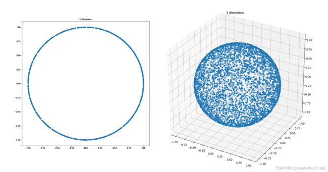
我们在二维和三维空间当中验证上述方法的有效性如下：

3. n维空间中两向量夹角考察

综上，我们即可对n维空间上的单位向量进行随机生成。

那么，我们就可以通过蒙特卡洛生成的方式来考察两个随机向量之间的夹角与维度n之间的变化关系。

我们给出结果图如下：

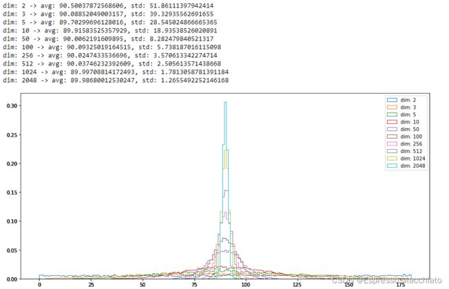
可以看到：

• 对于任意维度n，两个随机向量之间的夹角$\theta$的均值都是90度；
• 随着维度n的增加，夹角$\theta$的标准差分布逐渐减小，最终收敛到0，即在高维空间当中，两个向量的夹角将会非常接近于90度。

4. 总结 & 思考

综上，苏剑林在他的博客当中提到的这个结论就得到了证明，确实是一个非常有意思的结论。