Deep Cascaded Bi-Network for Face Hallucination--阅读笔记

1、We present a novel framework for hallucinating faces of unconstrained poses and with very low resolution (face size as small as 5pxIOD 1 ).

这篇文章呈现了一种可用于无约束姿态及非常低分辨率的人脸增强方法，人脸大小简单描述为两眼间像素的多少（最少的仅为5个像素）。

2、we alternatingly optimize two complementary tasks, namely face hallucination and dense correspondence field estimation, in a unified framework.

就是交替的优化两个任务：一个是普通的face hallucination ，一个是高密度区域估计。

3、In addition, we propose a new gated deep bi-network that contains two functionality-specialized branches to recover different levels of texture details. 

此外，本文还提出了一种门限bi-network，这个网络包含两个functionality-specialized分支，用于从各种纹理细节中恢复原图像信息。

4、 In this study, we extend the notion of prior to pixel-wise dense face correspondence field. 

这里提到的先验指的是：prior on face structure及 face spatial configuration，而本文就是扩展这种先验，利用像素级的高密度人脸对应区域（或许该翻译成密集响应区域？）。

5、Here the dense correspondence field is necessary for describing the spatial configuration for its pixel-wise (not by facial landmarks) and correspondence (not by face parsing)
properties.

密度响应区域用于描述像素级的空间结构及对应的属性。

6、

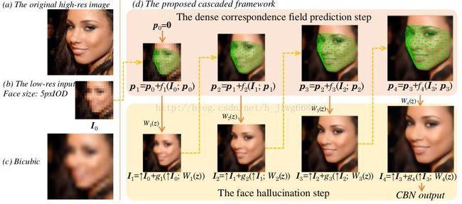
Fig. 1. (a) The original high-res image. (b) The low-res input with a size of 5pxIOD. (c) The result of bicubic interpolation. (d) An overview of the proposed face hallucination
framework. The solid arrows indicate the hallucination step that hallucinates the face with spatial cues, i.e. the dense correspondence field. The dashed arrows indicate the
spatial prediction step that estimates the dense correspondence field.

这里给出了原始高分辨率图片（a），低分辨率图片（b）眼间为5个像素，利用Bicubic插值得到的高分辨率图片（c），以及本文提及的框架（d）。其中实线箭头指示的是利用空间线索（例如密度响应区域）进行face hallucinates的结果，而虚线箭头指示的是重新估计密度响应区域。

7、Consequently, we face a chicken-and-egg problem - face hallucination is better guided by face spatial configuration, while the latter requires a high resolution face. This issue, however,has been mostly ignored or bypassed in previous works .

面对先有鸡还是先有蛋的问题，先前的研究工作都忽略了这一问题。

8、The two tasks at hand - the high-level face correspondence estimation and low-level face hallucination are complementary and can be alternatingly refined with the guidance from each other. 

本文提出的框架里的两个交替任务：高水平人脸区域估计及低层次的人脸hallucination.

9、During the cascade iteration, the dense correspondence field is progressively refined with the increasing face resolution, while the image resolution is adaptively upscaled guided by the finer dense correspondence field.

在两个任务交替执行过程中，密度响应区域随着人脸分辨率提高逐渐改善，而密度响应区域的改善也指引着图像分辨率自适应的提高。

10、To better recover different levels of texture details on faces, we propose a new gated deep bi-network architecture in the face hallucination step in each cascade.

为了从人脸的上更好的恢复不同层次的纹理细节，本文提出了门限bi-network架构，用于人脸hallucination阶段。

11、In contrast to aforementioned studies, the proposed network consists two functionality-specialized branches, which are trained end-to-end. The first branch, referred as common branch, conservatively recovers texture details that are only detectable from the low-res input, similar to general super resolution. The other branch, referred as high frequency branch,super-resolves faces with the additional high-frequency prior warped by the estimated face correspondence field in the current cascade. Thanks to the guidance of prior, this branch is capable of recovering and synthesizing un-revealed texture details in the overly low-res input image.

这里讲解了本文提出的网络的两个分支：common branch用以从低分辨率图像恢复纹理信息；high-frequency branch就是将估计的人脸响应区域的先验进行整合。通过这个先验的指导，这个branch可以恢复并合成在低分辨率图像中未显露出的纹理细节。

12、 A pixel-wise gate network is learned to fuse the results from the two branches. 

一种像素级的门限网络将两个分支进行整合。

13、Although the high-frequency branch synthesizes the facial parts that are occluded (the eyes with sun-glasses), the gate network automatically favours the results from the common branch during fusion.

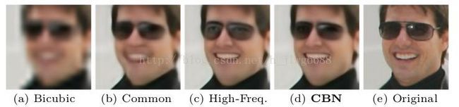
Fig. 2. Examples for visualizing the effects of the proposed gated deep bi-network. (a) The bicubic interpolation of the input. (b) Results where only common branches are
enabled. (c) Results where only high-frequency branches are enabled. (d) Results of the proposed CBN when both branches are enabled. (e) The original high-res image.
Best viewed by zooming in the electronic version.

（a）是Bicubic插值得到的结果，（b）是common branch的结果，（c）是high-freq branch的结果，（d）是两个branch结合的结果，可以看到（c）合成了被眼镜遮挡住的眼睛，然而在合并时门限网络自动的倾向于common branch的结果。

14、The facial image is denoted as a matrix I. We use x 2 R2 to denote the (x; y) coordinates of a pixel on I.

The dense face correspondence field defines a pixel-wise correspondence mapping from M ⊂ R 2 (the 2D face region in the mean face template) to the face region in image I. We represent the dense field with a warping function [38], x = W (z) : M → R 2 , which maps the coordinates z ∈ M from the mean shape template domain to the target coordinates x ∈ R 2 . See Fig. 3(a,b) for a clearillustration.

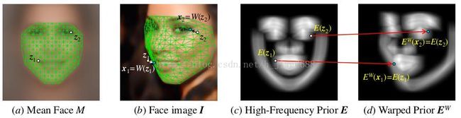
Fig. 3. (a,b) Illustration of the mean face template M and the facial image I. The grid denotes the dense correspondence field W (z). The warping from z to x is determined
by this warping function W (z). (c,d) Illustration of the high-frequency prior E and the prior after warping E W for the sample image in (b). Note that both E and E W have C channels. Each channel only contains one ‘contour line’. For the purpose of visualization, in this figure, we reduce their channel dimension to one channel with max operation. We leave out all indices k for clarity. Best viewed in the electronic version.

 文中所说的 密度人脸响应区域指的就是定义一个像素级的从中性人脸模板到指定图像I的像素级的映射：x=W（z）

15、Following [39], we model the warping residual W (z) − z as a linear combination of the dense facial deformation bases, i.e.

where denotes the deformation coefficients and B(z) =denotes the deformation bases. The N bases are chosen in the AAMs manner [40], that 4 out of N correspond to the similarity transform and the remaining for non-rigid deformations. Note that the bases are pre-defined and shared by all samples. Hence the dense field is actually controlled by the deformation coefficients p for each sample. When p = 0, the dense field equals to the mean face template.

这里解释如何得到这个W（z），其中p是参数，而B是由AAMs算法得到的变形基，这个基是预先得到的，并且由以后的所有图片共用的，因此密度区域完全由变形参数p来控制，特别的，当p=0时，密度区域等于平均人脸模型。

16、Our framework consists of K iterations (Fig. 1(d)). Each iteration updates the prediction via

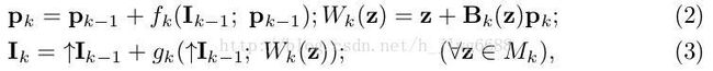
where k iterates from 1 to K. Here, Eq. 2 represents the dense field updating step while Eq. 3 stands for the spatially guided face hallucination step in each cascade. ‘↑’ denotes the upscaling process (2× upscaling with bicubic interpolation in our implementation).

这里给出了每次迭代时变形参数更新方式，密度人脸响应区域的更新方式，以及第k次上采样得到的高分辨率图片I的获得方式。

17、The framework starts from I 0 and p 0 . I 0 denotes the input low-res facial image. p 0 is a zero vector representing the deformation coefficients of the mean face template. The final hallucinated facial image output is I K .

也就是说整个系统从I(0)和p(0)开始，而I(0)就是输入的低分辨率人脸图像，p(0)是个0向量，最终的输出是图像I(k)。

18、Our model is composed of functions fk (dense field estimation) and gk (face hallucination with spatial cues). The deformation bases Bk are pre-defined for each cascade and fixed during the whole training and testing procedures. 

f函数用于密度区域估计，g函数用于空间线索的人脸hallucination，而B在每个级联阶段都预先设置的，在训练和测试阶段固定。

19、We train one gated bi-network for each cascade. For the k-th iteration, we take in the input image "Ik−1 and the current estimated dense correspondence field Wk(z), to predict the image residual G = Ik− "Ik−1.

对每一个级联都训练一个门限 bi-network网络，对于第k次迭代，输入为图像I(k-1)和当前的估计密度响应区域Wk(z)，结果就是预测图像残差。

20、we combine the two branches with a gate network. More precisely, if we denote the output from the common branch (A) and the high-frequency branch (B) as G A and GB respectively, we combine them with

where G denotes our predicted image residual I k − ↑I k−1 (i.e. the result of g k ), and G λ denotes the pixel-wise soft gate map that controls the combination of the two outputs G A and G B . We use ⊗ to denote element-wise multiplication.

common branch简称为GA，high-freq branch简称为GB，将这两个branch在门限网络中进行结合就是G，这个G也是I(k)和I(k-1)的残差，而Gλ标记为像素级的软门限映射，用以控制GA和GB的结合。

21、Figure 4 provides an overview of the gated bi-network architecture. Three convolutional sub-networks are designed to predict GA, GB and Gλ respectively. The common branch sub-network (blue in Fig. 4) takes in only the interpolated low-res image "Ik−1 to predict GA while the high-frequency branch sub-network (red in Fig. 4) takes in both "Ik−1 and the warped high-frequency prior EWk (warped according to the estimated dense correspondence field). All the inputs ("Ik−1 and EWk) as well as GA and GB are fed into the gate sub-network (cyan in Fig. 4) for predicting Gλ and the final high-res output G.

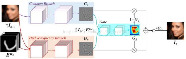
Fig. 4. Architecture of the proposed deep bi-network (for the k-th cascade). It consists of a common branch (blue), a high-frequency branch (red) and the gate network (cyan).

从图中可以看到GA、GB、Gλ三个网络的输入输出是什么。

//2017/5/2

22、人脸图像增强方面

We define high-frequency prior as the indication for location with high-frequency details.

就是定义高频先验为：高频细节位置的标记。

In this work, we generate high-frequency prior maps to enforce spatial guidance for hallucination.

产生这个高频先验图的目的就是为hallucination做空间指引。

The prior maps are obtained from the mean face template domain.

先验图从平均人脸模板获得。

for each training image, we compute the residual image between the original image ˆ I and the bicubic interpolation of I 0 , and then warp the residual map into the mean face
template domain.

对于每个训练图片，先计算原始图片和bicubic插值后的图片之间的残差图像，然后将残差图像扭曲成平均人脸模板。

We average the magnitude of the warped residual maps over all training images and form the preliminary high-frequency map.

对所有训练图像得到的扭曲的残差图取平均量级，最后形成初步的高频图。

To suppress the noise and provide a semantically meaningful prior, we cluster the preliminary high-frequency map into C continuous contours (10 in our implementation). We
form a C-channel maps, with each channel carrying one contour. We refer this C-channel maps as our high-frequency prior, and denote it as E k (z) : M k → R C . We use E k to represent E k (z) for all z ∈ M k . An illustration of the prior is shownin Fig. 3(c).

为了抑制噪声提供语义意义的先验，将初始高频图聚集成C个连续轮廓，形成一个C通道的图，每个通道就是一个轮廓，这个C通道图就是最终的高频先验，将它定义为Ek（z）。

23、For training the common branch, we use the following loss over all training samples

上面式子是common branch的损失函数。

The high-frequency branch has two inputs: ↑I k−1 and the warped high-frequency prior E W k (see Fig. 3(d) for illustration) to predict the output G B . The two inputs are fused in the channel dimension to form a (1 + C)-channel input. We use the following loss over all training samples

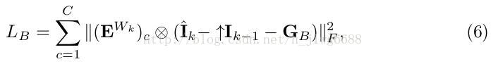
where denotes the c-th channel of the warped high-frequency prior maps. Compared to the common branch, we additionally utilize the prior knowledge as input and only penalize over the high-frequency area.

上面这个式子是high-pre branch的损失函数，并且只对对应的C个通道的部分进行惩罚。

Learning to predict the gate map G λ is supervised by the final loss

上面这式子是门限图的损失（最终损失）。

24、More precisely, we simultaneously obtain two sets of N deformation bases: B k (z) ∈ R 2×N for the dense field, and S k (l) ∈ R 2×N for the landmarks, where l is the landmark index. The bases for the dense field and landmarks are one-to-one related, i.e. both B k (z) and S k (l) share the same deformation coefficients p k ∈ R N :

where  denotes the coordinates of the l-th landmark, and denotes its mean location.

同时获得两个变形基（用变形系数P）

25、To predict the deformation coefficients p k in each cascade k, we utilize the powerful cascaded regression approach [23] for estimation. A Gauss-Newton steepest descent regression matrix R k is learned in each iteration k to map the observed appearance to the deformation coefficients update:

where φ is the shape-indexed feature [27,2] that concatenates the local appearance from all L landmarks, and φ  ̄ is its average over all the training samples.

为了在每个级联k预测变形系数p(k)，利用强大的级联的回归方法进行估计，该方法就是在每次迭代k，学习高斯-牛顿最徒下降回归矩阵R(x)，将观察得到的外观映射到变形系数更新。φ是shape-indexed 特征，用于连接所有的L个人脸标记和人脸局部外观，而φ  ̄ 则是全部训练样本的平均。

26、To learn the Gauss-Newton steepest descent regression matrix R k , we follow[23] to learn the Jacobian J k and then obtain R k via constructing the project-out Hessian:  . We refer readers to [23] for more details.

如何求解高斯-牛顿最速梯度下降矩阵。

27、