365天深度学习训练营-第P5周：运动鞋识别

• 本文为365天深度学习训练营 内部限免文章（版权归 K同学啊 所有）
• 参考文章地址： 第P4周：猴痘病识别 | 365天深度学习训练营
• 作者：K同学啊 | 接辅导、程序定制

我的环境：

• 语言环境：Python 3.6.8
• 编译器：jupyter notebook
• 深度学习环境：
  • torch==0.13.1、cuda==11.3
  • torchvision==1.12.1、cuda==11.3

一、前期工作

1. 设置 GPU

import torch
import torch.nn as nn
import torchvision
import torchvision.transforms as transforms
from torchvision import transforms, datasets

if __name__=='__main__':
    ''' 设置GPU '''
    device = torch.device("cuda" if torch.cuda.is_available() else "cpu")
    print("Using {} device\n".format(device))

Using cuda device

2. 导入数据

import os, PIL, pathlib
data_dir = 'D:/jupyter notebook/DL-100-days/datasets/46-data/'
data_dir = pathlib.Path(data_dir)
data_paths = list(data_dir.glob('*'))
classeNames = [str(path).split("\\")[5] for path in data_paths]
print(classeNames)

['test', 'train']

train_transforms = transforms.Compose([
    transforms.Resize([224, 224]),  # 将输入图片resize成统一尺寸
    # transforms.RandomHorizontalFlip(), # 随机水平翻转
    transforms.ToTensor(),          # 将PIL Image或numpy.ndarray转换为tensor，并归一化到[0,1]之间
    transforms.Normalize(           # 标准化处理-->转换为标准正太分布（高斯分布），使模型更容易收敛
        mean=[0.485, 0.456, 0.406],
        std=[0.229, 0.224, 0.225])  # 其中 mean=[0.485,0.456,0.406]与std=[0.229,0.224,0.225] 从数据集中随机抽样计算得到的。
])
 
test_transform = transforms.Compose([
    transforms.Resize([224, 224]),  # 将输入图片resize成统一尺寸
    transforms.ToTensor(),          # 将PIL Image或numpy.ndarray转换为tensor，并归一化到[0,1]之间
    transforms.Normalize(           # 标准化处理-->转换为标准正太分布（高斯分布），使模型更容易收敛
        mean=[0.485, 0.456, 0.406],
        std=[0.229, 0.224, 0.225])  # 其中 mean=[0.485,0.456,0.406]与std=[0.229,0.224,0.225] 从数据集中随机抽样计算得到的。
])
 
train_dataset = datasets.ImageFolder("D:/jupyter notebook/DL-100-days/datasets/46-data/train/",transform=train_transforms)
test_dataset  = datasets.ImageFolder("D:/jupyter notebook/DL-100-days/datasets/46-data/test/",transform=train_transforms)
 
print(train_dataset.class_to_idx)

{'adidas': 0, 'nike': 1}

3. 划分数据集

batch_size = 32
 
train_dl = torch.utils.data.DataLoader(train_dataset,
                                           batch_size=batch_size,
                                           shuffle=True,
                                           num_workers=1) 
test_dl = torch.utils.data.DataLoader(test_dataset,
                                          batch_size=batch_size,
                                          shuffle=True,
                                          num_workers=1)
 
for X, y in test_dl:
    print("Shape of X [N, C, H, W]: ", X.shape)
    print("Shape of y: ", y.shape, y.dtype)
    break

Shape of X [N, C, H, W]: torch.Size([32, 3, 224, 224])
Shape of y: torch.Size([32]) torch.int64

二、构建简单的CNN网络

import torch.nn.functional as F
class Model(nn.Module):
    def __init__(self):
        super(Model, self).__init__()
        self.conv1 = nn.Sequential(
            nn.Conv2d(3, 12, kernel_size=5, padding=0),  #3,12为输入输出通道数量 12*220*220
            nn.BatchNorm2d(12),
            nn.ReLU())
 
        self.conv2 = nn.Sequential(
            nn.Conv2d(12, 12, kernel_size=5, padding=0),  # 12*216*216
            nn.BatchNorm2d(12),
            nn.ReLU())
 
        self.pool3 = nn.Sequential(
            nn.MaxPool2d(2))  # 12*108*108
 
        self.conv4 = nn.Sequential(
            nn.Conv2d(12, 24, kernel_size=5, padding=0),  # 24*104*104
            nn.BatchNorm2d(24),
            nn.ReLU())
 
        self.conv5 = nn.Sequential(
            nn.Conv2d(24, 24, kernel_size=5, padding=0),  # 24*100*100
            nn.BatchNorm2d(24),
            nn.ReLU())
 
        self.pool6 = nn.Sequential(
            nn.MaxPool2d(2))  # 24*50*50
 
        self.dropout = nn.Sequential(
            nn.Dropout(0.2))
 
        self.fc = nn.Sequential(
            nn.Linear(24 * 50 * 50, len(classeNames)))
 
    def forward(self, x):
        batch_size = x.size(0)
        x = self.conv1(x)  # 卷积-BN-激活
        x = self.conv2(x)  # 卷积-BN-激活
        x = self.pool3(x)  # 池化
        x = self.conv4(x)  # 卷积-BN-激活
        x = self.conv5(x)  # 卷积-BN-激活
        x = self.pool6(x)  # 池化
        x = self.dropout(x)
        x = x.view(batch_size, -1)  # flatten 变成全连接网络需要的输入 (batch, 24*50*50) ==> (batch, -1), -1 此处自动算出的是24*50*50
        x = self.fc(x)
 
        return x
 
 
device = "cuda" if torch.cuda.is_available() else "cpu"
print("Using {} device".format(device))
 
model = Model().to(device)
print(model)

Using cuda device
Model(
  (conv1): Sequential(
    (0): Conv2d(3, 12, kernel_size=(5, 5), stride=(1, 1))
    (1): BatchNorm2d(12, eps=1e-05, momentum=0.1, affine=True, track_running_stats=True)
    (2): ReLU()
  )
  (conv2): Sequential(
    (0): Conv2d(12, 12, kernel_size=(5, 5), stride=(1, 1))
    (1): BatchNorm2d(12, eps=1e-05, momentum=0.1, affine=True, track_running_stats=True)
    (2): ReLU()
  )
  (pool3): Sequential(
    (0): MaxPool2d(kernel_size=2, stride=2, padding=0, dilation=1, ceil_mode=False)
  )
  (conv4): Sequential(
    (0): Conv2d(12, 24, kernel_size=(5, 5), stride=(1, 1))
    (1): BatchNorm2d(24, eps=1e-05, momentum=0.1, affine=True, track_running_stats=True)
    (2): ReLU()
  )
  (conv5): Sequential(
    (0): Conv2d(24, 24, kernel_size=(5, 5), stride=(1, 1))
    (1): BatchNorm2d(24, eps=1e-05, momentum=0.1, affine=True, track_running_stats=True)
    (2): ReLU()
  )
  (pool6): Sequential(
    (0): MaxPool2d(kernel_size=2, stride=2, padding=0, dilation=1, ceil_mode=False)
  )
  (dropout): Sequential(
    (0): Dropout(p=0.2, inplace=False)
  )
  (fc): Sequential(
    (0): Linear(in_features=60000, out_features=2, bias=True)
  )
)

三、训练模型

1. 设置超参数

learn_rate = 1e-4 # 初始学习率
optimizer  = torch.optim.SGD(model.parameters(), lr=learn_rate)
loss_fn = nn.CrossEntropyLoss() # 创建损失函数

2. 编写训练函数

# 训练循环
def train(dataloader, model, loss_fn, optimizer):
    size = len(dataloader.dataset)  # 训练集的大小
    num_batches = len(dataloader)   # 批次数目, (size/batch_size，向上取整)
 
    train_loss, train_acc = 0, 0  # 初始化训练损失和正确率
    
    for X, y in dataloader:  # 获取图片及其标签
        X, y = X.to(device), y.to(device)
        
        # 计算预测误差
        pred = model(X)          # 网络输出
        loss = loss_fn(pred, y)  # 计算网络输出和真实值之间的差距，targets为真实值，计算二者差值即为损失
        
        # 反向传播
        optimizer.zero_grad()  # grad属性归零
        loss.backward()        # 反向传播
        optimizer.step()       # 每一步自动更新
        
        # 记录acc与loss
        train_acc  += (pred.argmax(1) == y).type(torch.float).sum().item()
        train_loss += loss.item()
            
    train_acc  /= size
    train_loss /= num_batches
 
    return train_acc, train_loss

3. 编写测试函数

def test(dataloader, model, loss_fn):
    size = len(dataloader.dataset)  # 测试集的大小
    num_batches = len(dataloader)  # 批次数目
    test_loss, test_acc = 0, 0
 
    # 当不进行训练时，停止梯度更新，节省计算内存消耗
    with torch.no_grad():
        for imgs, target in dataloader:
            imgs, target = imgs.to(device), target.to(device)
 
            # 计算loss
            target_pred = model(imgs)
            loss = loss_fn(target_pred, target)
 
            test_loss += loss.item()
            test_acc += (target_pred.argmax(1) == target).type(torch.float).sum().item()
 
    test_acc /= size
    test_loss /= num_batches
 
    return test_acc, test_loss

def adjust_learning_rate(optimizer, epoch, start_lr):
    # 每2轮epoch衰减到原来的 0.92
    lr = start_lr * (0.92 ** (epoch // 2))
    for param_group in optimizer.param_groups:
        param_group['lr'] = lr

4. 正式训练

epochs     = 40
 
train_loss = []
train_acc  = []
test_loss  = []
test_acc   = []
 
for epoch in range(epochs):
    # 更新学习率（使用自定义学习率时使用）
    adjust_learning_rate(optimizer, epoch, learn_rate)
    
    model.train()
    epoch_train_acc, epoch_train_loss = train(train_dl, model, loss_fn, optimizer)
    # scheduler.step() # 更新学习率（调用官方动态学习率接口时使用）
    
    model.eval()
    epoch_test_acc, epoch_test_loss = test(test_dl, model, loss_fn)
    
    train_acc.append(epoch_train_acc)
    train_loss.append(epoch_train_loss)
    test_acc.append(epoch_test_acc)
    test_loss.append(epoch_test_loss)
    
    # 获取当前的学习率
    lr = optimizer.state_dict()['param_groups'][0]['lr']
    
    template = ('Epoch:{:2d}, Train_acc:{:.1f}%, Train_loss:{:.3f}, Test_acc:{:.1f}%, Test_loss:{:.3f}, Lr:{:.2E}')
    print(template.format(epoch+1, epoch_train_acc*100, epoch_train_loss, 
                          epoch_test_acc*100, epoch_test_loss, lr))
print('Done')

Epoch: 1, Train_acc:54.4%, Train_loss:0.794, Test_acc:56.6%, Test_loss:0.683, Lr:1.00E-04
Epoch: 2, Train_acc:67.1%, Train_loss:0.661, Test_acc:57.9%, Test_loss:0.646, Lr:1.00E-04
Epoch: 3, Train_acc:73.5%, Train_loss:0.577, Test_acc:65.8%, Test_loss:0.592, Lr:9.20E-05
Epoch: 4, Train_acc:72.3%, Train_loss:0.546, Test_acc:60.5%, Test_loss:0.642, Lr:9.20E-05
Epoch: 5, Train_acc:76.7%, Train_loss:0.514, Test_acc:71.1%, Test_loss:0.594, Lr:8.46E-05
Epoch: 6, Train_acc:76.5%, Train_loss:0.497, Test_acc:69.7%, Test_loss:0.575, Lr:8.46E-05
Epoch: 7, Train_acc:83.5%, Train_loss:0.460, Test_acc:72.4%, Test_loss:0.510, Lr:7.79E-05
Epoch: 8, Train_acc:82.5%, Train_loss:0.450, Test_acc:71.1%, Test_loss:0.544, Lr:7.79E-05
Epoch: 9, Train_acc:84.7%, Train_loss:0.418, Test_acc:72.4%, Test_loss:0.511, Lr:7.16E-05
Epoch:10, Train_acc:84.1%, Train_loss:0.413, Test_acc:73.7%, Test_loss:0.513, Lr:7.16E-05
Epoch:11, Train_acc:85.1%, Train_loss:0.402, Test_acc:75.0%, Test_loss:0.483, Lr:6.59E-05
Epoch:12, Train_acc:88.8%, Train_loss:0.375, Test_acc:72.4%, Test_loss:0.482, Lr:6.59E-05
Epoch:13, Train_acc:89.8%, Train_loss:0.363, Test_acc:77.6%, Test_loss:0.468, Lr:6.06E-05
Epoch:14, Train_acc:88.0%, Train_loss:0.364, Test_acc:68.4%, Test_loss:0.541, Lr:6.06E-05
Epoch:15, Train_acc:90.8%, Train_loss:0.344, Test_acc:77.6%, Test_loss:0.509, Lr:5.58E-05
Epoch:16, Train_acc:91.0%, Train_loss:0.334, Test_acc:73.7%, Test_loss:0.478, Lr:5.58E-05
Epoch:17, Train_acc:90.2%, Train_loss:0.341, Test_acc:76.3%, Test_loss:0.458, Lr:5.13E-05
Epoch:18, Train_acc:90.2%, Train_loss:0.317, Test_acc:80.3%, Test_loss:0.461, Lr:5.13E-05
Epoch:19, Train_acc:91.6%, Train_loss:0.326, Test_acc:78.9%, Test_loss:0.466, Lr:4.72E-05
Epoch:20, Train_acc:92.6%, Train_loss:0.308, Test_acc:78.9%, Test_loss:0.500, Lr:4.72E-05
Epoch:21, Train_acc:93.4%, Train_loss:0.301, Test_acc:81.6%, Test_loss:0.476, Lr:4.34E-05
Epoch:22, Train_acc:93.4%, Train_loss:0.288, Test_acc:82.9%, Test_loss:0.437, Lr:4.34E-05
Epoch:23, Train_acc:93.2%, Train_loss:0.301, Test_acc:80.3%, Test_loss:0.509, Lr:4.00E-05
Epoch:24, Train_acc:94.2%, Train_loss:0.293, Test_acc:78.9%, Test_loss:0.450, Lr:4.00E-05
Epoch:25, Train_acc:94.6%, Train_loss:0.283, Test_acc:78.9%, Test_loss:0.479, Lr:3.68E-05
Epoch:26, Train_acc:94.2%, Train_loss:0.283, Test_acc:81.6%, Test_loss:0.429, Lr:3.68E-05
Epoch:27, Train_acc:93.2%, Train_loss:0.287, Test_acc:80.3%, Test_loss:0.466, Lr:3.38E-05
Epoch:28, Train_acc:95.0%, Train_loss:0.273, Test_acc:81.6%, Test_loss:0.454, Lr:3.38E-05
Epoch:29, Train_acc:95.0%, Train_loss:0.271, Test_acc:80.3%, Test_loss:0.422, Lr:3.11E-05
Epoch:30, Train_acc:95.0%, Train_loss:0.274, Test_acc:78.9%, Test_loss:0.413, Lr:3.11E-05
Epoch:31, Train_acc:94.8%, Train_loss:0.262, Test_acc:82.9%, Test_loss:0.453, Lr:2.86E-05
Epoch:32, Train_acc:94.4%, Train_loss:0.272, Test_acc:81.6%, Test_loss:0.457, Lr:2.86E-05
Epoch:33, Train_acc:95.2%, Train_loss:0.266, Test_acc:81.6%, Test_loss:0.401, Lr:2.63E-05
Epoch:34, Train_acc:95.8%, Train_loss:0.255, Test_acc:81.6%, Test_loss:0.453, Lr:2.63E-05
Epoch:35, Train_acc:95.2%, Train_loss:0.261, Test_acc:82.9%, Test_loss:0.472, Lr:2.42E-05
Epoch:36, Train_acc:95.8%, Train_loss:0.245, Test_acc:78.9%, Test_loss:0.423, Lr:2.42E-05
Epoch:37, Train_acc:95.2%, Train_loss:0.249, Test_acc:81.6%, Test_loss:0.447, Lr:2.23E-05
Epoch:38, Train_acc:96.0%, Train_loss:0.255, Test_acc:81.6%, Test_loss:0.458, Lr:2.23E-05
Epoch:39, Train_acc:95.0%, Train_loss:0.247, Test_acc:80.3%, Test_loss:0.423, Lr:2.05E-05
Epoch:40, Train_acc:94.4%, Train_loss:0.252, Test_acc:80.3%, Test_loss:0.451, Lr:2.05E-05
Done

# 模型保存
PATH = 'D:/jupyter notebook/DL-100-days/datasets/46-data/model.pth'  # 保存的参数文件名
torch.save(model.state_dict(), PATH)
 
# 将参数加载到model当中
model.load_state_dict(torch.load(PATH, map_location=device))

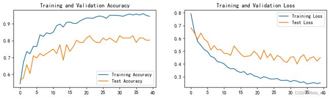
四、结果可视化

1.Loss 与 Accuracy 图

import matplotlib.pyplot as plt
#隐藏警告
import warnings
warnings.filterwarnings("ignore")               #忽略警告信息
plt.rcParams['font.sans-serif']    = ['SimHei'] # 用来正常显示中文标签
plt.rcParams['axes.unicode_minus'] = False      # 用来正常显示负号
plt.rcParams['figure.dpi']         = 100        #分辨率
 
epochs_range = range(epochs)
 
plt.figure(figsize=(12, 3))
plt.subplot(1, 2, 1)
 
plt.plot(epochs_range, train_acc, label='Training Accuracy')
plt.plot(epochs_range, test_acc, label='Test Accuracy')
plt.legend(loc='lower right')
plt.title('Training and Validation Accuracy')
 
plt.subplot(1, 2, 2)
plt.plot(epochs_range, train_loss, label='Training Loss')
plt.plot(epochs_range, test_loss, label='Test Loss')
plt.legend(loc='upper right')
plt.title('Training and Validation Loss')
plt.show()

2.指定图片进行预测

from PIL import Image
 
classes = list(train_dataset.class_to_idx)
def predict_one_image(image_path, model, transform, classes):
    test_img = Image.open(image_path).convert('RGB')
    #plt.imshow(test_img)  # 展示预测的图片
 
    test_img = transform(test_img)
    img = test_img.to(device).unsqueeze(0)  # （0表示，在第一个位置增加维度）
 
    model.eval()
    output = model(img)
 
    _, pred = torch.max(output, 1)
    pred_class = classes[pred]
    print(f'预测结果是：{pred_class}')
    # 预测训练集中的某张照片
 
 
predict_one_image(image_path='D:/jupyter notebook/DL-100-days/datasets/46-data/test/adidas/9.jpg',
                  model=model,
                  transform=train_transforms,
                  classes=classes)

预测结果是：Adidas