【cs231n Assignment1】SVM
个人学习笔记
date:2023.01.03
Goals
- Implement and apply a Multiclass Support Vector Machine (SVM) classifier.
- 完成并应用多分类SVM分类器
Data Loading and Preprocessing
(一)载入图像数据 \color{purple}(一)载入图像数据 (一)载入图像数据
# Load the raw CIFAR-10 data.
cifar10_dir = 'cs231n/datasets/cifar-10-batches-py'

# Cleaning up variables to prevent loading data multiple times (which may cause memory issue)
try:
   del X_train, y_train
   del X_test, y_test
   print('Clear previously loaded data.')
except:
   pass

X_train, y_train, X_test, y_test = load_CIFAR10(cifar10_dir)

# As a sanity check, we print out the size of the training and test data.
print('Training data shape: ', X_train.shape)
print('Training labels shape: ', y_train.shape)
print('Test data shape: ', X_test.shape)
print('Test labels shape: ', y_test.shape)

#Training data shape:  (50000, 32, 32, 3)
#Training labels shape:  (50000,)
#Test data shape:  (10000, 32, 32, 3)
#Test labels shape:  (10000,)
(二)数据分类 \color{purple}(二)数据分类 (二)数据分类
将数据分类为训练集、验证集、测试集以及development 集(开发集?)
开发集是一组在模型开发过程中使用的数据,但不用于训练或评估模型。它可以用来微调模型,例如调整超参数,或在将新想法加入模型之前尝试它们。由于不用于训练或评估模型,开发集可以更准确地评估模型在新数据上的性能。
# Split the data into train, val, and test sets. In addition we will
# create a small development set as a subset of the training data;
# we can use this for development so our code runs faster.
num_training = 49000
num_validation = 1000
num_test = 1000
num_dev = 500

# Our validation set will be num_validation points from the original
# training set.
mask = range(num_training, num_training + num_validation)
X_val = X_train[mask]
y_val = y_train[mask]

# Our training set will be the first num_train points from the original
# training set.
mask = range(num_training)
X_train = X_train[mask]
y_train = y_train[mask]

# We will also make a development set, which is a small subset of
# the training set.
mask = np.random.choice(num_training, num_dev, replace=False)
X_dev = X_train[mask]
y_dev = y_train[mask]

# We use the first num_test points of the original test set as our
# test set.
mask = range(num_test)
X_test = X_test[mask]
y_test = y_test[mask]

print('Train data shape: ', X_train.shape)
print('Train labels shape: ', y_train.shape)
print('Validation data shape: ', X_val.shape)
print('Validation labels shape: ', y_val.shape)
print('Test data shape: ', X_test.shape)
print('Test labels shape: ', y_test.shape)

#Train data shape:  (49000, 32, 32, 3)
#Train labels shape:  (49000,)
#Validation data shape:  (1000, 32, 32, 3)
#Validation labels shape:  (1000,)
#Test data shape:  (1000, 32, 32, 3)
#Test labels shape:  (1000,)
要点:
- 将训练集分为训练集和验证集,训练集为前49000个图像,验证集为后1000个图像
- 使用
np.random.choice(arr,num,replace=False)函数在训练集上随机选取开发集
(三)将图像数据转换为行向量 \color{purple}(三) 将图像数据转换为行向量 (三)将图像数据转换为行向量
# Preprocessing: reshape the image data into rows
X_train = np.reshape(X_train, (X_train.shape[0], -1))
X_val = np.reshape(X_val, (X_val.shape[0], -1))
X_test = np.reshape(X_test, (X_test.shape[0], -1))
X_dev = np.reshape(X_dev, (X_dev.shape[0], -1))

# As a sanity check, print out the shapes of the data
print('Training data shape: ', X_train.shape)
print('Validation data shape: ', X_val.shape)
print('Test data shape: ', X_test.shape)
print('dev data shape: ', X_dev.shape)
#Training data shape:  (49000, 3072)
#Validation data shape:  (1000, 3072)
#Test data shape:  (1000, 3072)
#dev data shape:  (500, 3072)
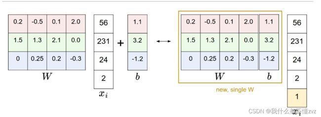
(四)图像减去均值并加上 b i a s t e r m 列 \color{purple}(四) 图像减去均值并加上bias\space term列 (四)图像减去均值并加上bias term列
参考:https://blog.csdn.net/qq_32172681/article/details/102455225
图像在每个样本上减去数据的统计平均值可以移除共同的部分,凸显个体差异。并且应该只在训练集中减去均值,因为深度学习原则是我们获取的数据应全部来自训练集。
# Preprocessing: subtract the mean image
# first: compute the image mean based on the training data
mean_image = np.mean(X_train, axis=0)
print(mean_image[:10]) # print a few of the elements
print(mean_image.shape)
plt.figure(figsize=(4,4))
plt.imshow(mean_image.reshape((32,32,3)).astype('uint8')) # visualize the mean image
plt.show()

# second: subtract the mean image from train and test data
X_train -= mean_image
X_val -= mean_image
X_test -= mean_image
X_dev -= mean_image

# third: append the bias dimension of ones (i.e. bias trick) so that our SVM
# only has to worry about optimizing a single weight matrix W.
X_train = np.hstack([X_train, np.ones((X_train.shape[0], 1))])
X_val = np.hstack([X_val, np.ones((X_val.shape[0], 1))])
X_test = np.hstack([X_test, np.ones((X_test.shape[0], 1))])
X_dev = np.hstack([X_dev, np.ones((X_dev.shape[0], 1))])

print(X_train.shape, X_val.shape, X_test.shape, X_dev.shape)
要点:
- 使用
np.mean(arr,axis=0)计算每一列的均值,就是所有图像在同一个像素的均值,所以返回的结果应是(3072,) 意味着3072个像素的均值 - 使用
np.hstack([arr1,arr2])来进行水平方向的拼接,拼接后返回矩阵的列数应为3073 - bias term列置为1,原理如下图所示,展开为列向量时末尾为1,乘上bias term时就不会改变什么。
均值image效果如下:(所有图像的公共部分)

SVM classifier
(一)损失函数 \color{purple}(一) 损失函数 (一)损失函数
回顾一下SVM损失函数公式:( s j s_j sj为正确结果得分)
L i = 1 N ∑ j ≠ y i m a x ( 0 , s j − s y i + Δ ) L_{i} =\frac{1}{N}\sum_{j\not = y_{i}}max(0,s_j-s_{y_{i}}+\Delta) Li=N1j=yi∑max(0,sj−syi+Δ)
计算损失函数, X i ⋅ W X_{i}·W Xi⋅W得到第 i i i个样本各个分类的得分,结合 y i y_i yi得出正确结果得分 s y i s_{y_i} syi, s j s_j sj为其他类别得分。运用公式算出该图像的损失函数值。
ps. X为[500,3073], W为[3073,10],Y为[3073,]
def svm_loss_naive(W, X, y, reg):
    """
    Structured SVM loss function, naive implementation (with loops).

    Inputs have dimension D, there are C classes, and we operate on minibatches
    of N examples.

    Inputs:
    - W: A numpy array of shape (D, C) containing weights.
    - X: A numpy array of shape (N, D) containing a minibatch of data.
    - y: A numpy array of shape (N,) containing training labels; y[i] = c means
      that X[i] has label c, where 0 <= c < C.
    - reg: (float) regularization strength

    Returns a tuple of:
    - loss as single float
    - gradient with respect to weights W; an array of same shape as W
    """
    dW = np.zeros(W.shape)  # initialize the gradient as zero,3072,10

    # compute the loss and the gradient
    num_classes = W.shape[1] #10
    num_train = X.shape[0] #500
    loss = 0.0
    for i in range(num_train):
        scores = X[i].dot(W) #[i,3073]*[3073,10]
        #表示第i个样本,10个分类得分
        correct_class_score = scores[y[i]] #该样本正确分类得分
        for j in range(num_classes):
            if j == y[i]:
                continue
            margin = scores[j] - correct_class_score + 1  # note delta = 1
            if margin > 0:
                loss += margin

    # Right now the loss is a sum over all training examples, but we want it
    # to be an average instead so we divide by num_train.
    loss /= num_train

    # Add regularization to the loss.
    loss += reg * np.sum(W * W)
要点:
- 得分为图像 X i X_i Xi与 W W W的点积([i,3073]*[3073,10] = [i,10] 表示第 i i i个样本10个分类得分)
- 使用循环,套用公式
- 求平均值
- 加上L2正则项
loss += reg * np.sum(W * W)
(二)梯度 \color{purple}(二) 梯度 (二)梯度
由损失函数表达式
L i = 1 N ∑ j ≠ y i m a x ( 0 , s j − s y i + Δ ) L_{i} =\frac{1}{N}\sum_{j\not = y_{i}}max(0,s_j-s_{y_{i}}+\Delta) Li=N1j=yi∑max(0,sj−syi+Δ)
可得 j ! = y i j!=y_i j!=yi 时梯度表达式
∂ L i ∂ s j = 1 ( i f j ≠ y i A n d s j − s y i + Δ > 0 ) ∂ L i ∂ s j = 0 ( O t h e r c o n d i t i o n ) \frac{\partial{L_i}}{\partial{s_j}} = 1(if \space j\not =y_i \space And \space s_j-s_{y_i}+\Delta>0)\\\frac{\partial{L_i}}{\partial{s_j}} = 0(Other\space condition) ∂sj∂Li=1(if j=yi And sj−syi+Δ>0)∂sj∂Li=0(Other condition)
又有scores表达式 s = X [ i ] ∗ W s = X[i]*W s=X[i]∗W,可知权重矩阵梯度为
∂ s j ∂ W = X [ i ] , ∂ L i ∂ W = X [ i ] ∗ 1 \frac{\partial{s_j}}{\partial{W}}=X[i],\space\frac{\partial{L_i}}{\partial{W}}=X[i]*1 ∂W∂sj=X[i], ∂W∂Li=X[i]∗1
同理的, j = y i j=y_i j=yi 时的梯度表达式为
∂ L i ∂ s y i = − 1 ( i f j = i A n d s j − s y i + Δ > 0 ) \frac{\partial{L_i}}{\partial{s_{y_i}}} = -1(if \space j =i \space And \space s_j-s_{y_i}+\Delta>0) ∂syi∂Li=−1(if j=i And sj−syi+Δ>0)
权重矩阵梯度表达式为,权重矩阵梯度为该值的累加
∂ s y i ∂ W = X [ i ] , ∂ L i ∂ W = − X [ i ] \frac{\partial{s_{y_i}}}{\partial{W}}=X[i],\space\frac{\partial{L_i}}{\partial{W}}=-X[i] ∂W∂syi=X[i], ∂W∂Li=−X[i]
故梯度计算代码如下:
    dW = np.zeros(W.shape) # initialize the gradient as zero

    # compute the loss and the gradient
    num_classes = W.shape[1]
    num_train = X.shape[0]
    loss = 0.0
    for i in range(num_train):
        f=0
        scores = X[i].dot(W)
        correct_class_score = scores[y[i]]
        for j in range(num_classes):
            if j == y[i]:
                continue
            margin = scores[j] - correct_class_score + 1 # note delta = 1
            if margin > 0:
                loss += margin
                dW[:,j]+=X[i]
                f+=1
        dW[:,y[i]] += -f*X[i]

    # Right now the loss is a sum over all training examples, but we want it
    # to be an average instead so we divide by num_train.
    loss /= num_train
    dW/=num_train

    # Add regularization to the loss.
    loss += reg * np.sum(W * W)

    #############################################################################
    # TODO:                                                                     #
    # Compute the gradient of the loss function and store it dW.                #
    # Rather that first computing the loss and then computing the derivative,   #
    # it may be simpler to compute the derivative at the same time that the     #
    # loss is being computed. As a result you may need to modify some of the    #
    # code above to compute the gradient.                                       #
    #############################################################################
    # *****START OF YOUR CODE (DO NOT DELETE/MODIFY THIS LINE)*****

    dW+=2*reg*W

    # *****END OF YOUR CODE (DO NOT DELETE/MODIFY THIS LINE)*****
要点:
- loss函数的正则项为L2正则
- 权重矩阵的正则项为L1正则(稀疏矩阵狂喜)
以下为向量化(很巧,细品)
def svm_loss_vectorized(W, X, y, reg):
    """
    Structured SVM loss function, vectorized implementation.

    Inputs and outputs are the same as svm_loss_naive.
    """
    loss = 0.0
    dW = np.zeros(W.shape)  # initialize the gradient as zero

    #############################################################################
    # TODO:                                                                     #
    # Implement a vectorized version of the structured SVM loss, storing the    #
    # result in loss.                                                           #
    #############################################################################
    # *****START OF YOUR CODE (DO NOT DELETE/MODIFY THIS LINE)*****

    n = len(X) #500
    scores = X.dot(W) # 500*10
    correct_scores = scores[np.arange(scores),y] #(500,)
    margin = np.clip(scores-correct_scores.reshape([-1,1])+1,0,None) #margin(500,10),加上bias term
    margin[np.arange(n),y] = 0 # 正确分类损失值设为0,
    loss = np.sum(margin)/n + reg*np.sum(np.square(W))


    # *****END OF YOUR CODE (DO NOT DELETE/MODIFY THIS LINE)*****

    #############################################################################
    # TODO:                                                                     #
    # Implement a vectorized version of the gradient for the structured SVM     #
    # loss, storing the result in dW.                                           #
    #                                                                           #
    # Hint: Instead of computing the gradient from scratch, it may be easier    #
    # to reuse some of the intermediate values that you used to compute the     #
    # loss.                                                                     #
    #############################################################################
    # *****START OF YOUR CODE (DO NOT DELETE/MODIFY THIS LINE)*****

    m = (margin>0).astype(int) #大于0的设为1,否则为0
    f = np.sum(m,axis=1) #每一行大于0的个数
    m[np.arange(n),y] -= f
    dW = X.T.dot(m)/n + 2*reg*W  #W (3073,10) X(500,3073) m(500,10)


    # *****END OF YOUR CODE (DO NOT DELETE/MODIFY THIS LINE)*****

    return loss, dW
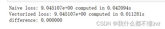
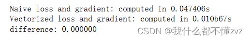
数据检查:

内嵌问题1:
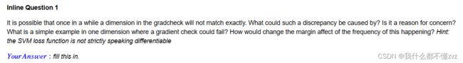
答案: 当正确类型分数大于等于错误类型分数加上margin时,将测不出损失值,这也是主要原因。
时间比对:
使用mini-batch并更新权重
class LinearClassifier(object):
    def __init__(self):
        self.W = None

    def train(
        self,
        X,
        y,
        learning_rate=1e-3,
        reg=1e-5,
        num_iters=100,
        batch_size=200,
        verbose=False,
    ):
        """
        Train this linear classifier using stochastic gradient descent.

        Inputs:
        - X: A numpy array of shape (N, D) containing training data; there are N
          training samples each of dimension D.
        - y: A numpy array of shape (N,) containing training labels; y[i] = c
          means that X[i] has label 0 <= c < C for C classes.
        - learning_rate: (float) learning rate for optimization.
        - reg: (float) regularization strength.
        - num_iters: (integer) number of steps to take when optimizing
        - batch_size: (integer) number of training examples to use at each step.
        - verbose: (boolean) If true, print progress during optimization.

        Outputs:
        A list containing the value of the loss function at each training iteration.
        """
        num_train, dim = X.shape
        num_classes = (
            np.max(y) + 1
        )  # assume y takes values 0...K-1 where K is number of classes
        if self.W is None:
            # lazily initialize W
            self.W = 0.001 * np.random.randn(dim, num_classes)

        # Run stochastic gradient descent to optimize W
        loss_history = []
        for it in range(num_iters):
            X_batch = None
            y_batch = None

            #########################################################################
            # TODO:                                                                 #
            # Sample batch_size elements from the training data and their           #
            # corresponding labels to use in this round of gradient descent.        #
            # Store the data in X_batch and their corresponding labels in           #
            # y_batch; after sampling X_batch should have shape (batch_size, dim)   #
            # and y_batch should have shape (batch_size,)                           #
            #                                                                       #
            # Hint: Use np.random.choice to generate indices. Sampling with         #
            # replacement is faster than sampling without replacement.              #
            #########################################################################
            # *****START OF YOUR CODE (DO NOT DELETE/MODIFY THIS LINE)*****

            indx = np.random.choice(num_train,size=batch_size,replace=True)
            X_batch = X[indx,:]
            y_batch = y[indx]

            # *****END OF YOUR CODE (DO NOT DELETE/MODIFY THIS LINE)*****

            # evaluate loss and gradient
            loss, grad = self.loss(X_batch, y_batch, reg)
            loss_history.append(loss)

            # perform parameter update
            #########################################################################
            # TODO:                                                                 #
            # Update the weights using the gradient and the learning rate.          #
            #########################################################################
            # *****START OF YOUR CODE (DO NOT DELETE/MODIFY THIS LINE)*****

            self.W += -learning_rate*grad

            # *****END OF YOUR CODE (DO NOT DELETE/MODIFY THIS LINE)*****

            if verbose and it % 100 == 0:
                print("iteration %d / %d: loss %f" % (it, num_iters, loss))

        return loss_history
要点:
- 使用
np.random.choice(arr,size=,replace=True)随机选取 - 更新参数
self.W += -learning_rate*grad
损失值可视化
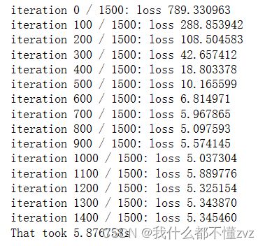
from cs231n.classifiers import LinearSVM
svm = LinearSVM()
tic = time.time()
loss_hist = svm.train(X_train, y_train, learning_rate=1e-7, reg=2.5e4,
                      num_iters=1500, verbose=True)
toc = time.time()
print('That took %fs' % (toc - tic))
作图:
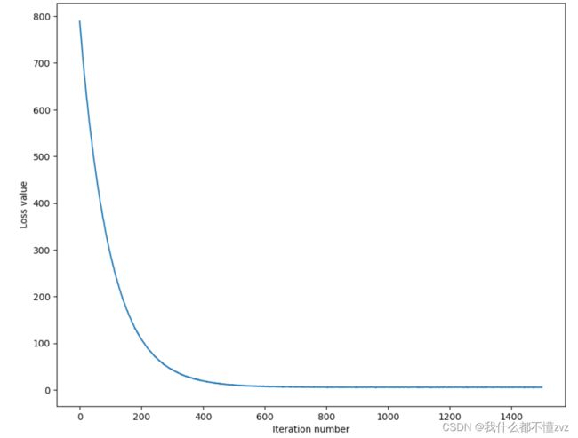
# A useful debugging strategy is to plot the loss as a function of
# iteration number:
plt.plot(loss_hist)
plt.xlabel('Iteration number')
plt.ylabel('Loss value')
plt.show()
预测结果
    def predict(self, X):
        """
        Use the trained weights of this linear classifier to predict labels for
        data points.

        Inputs:
        - X: A numpy array of shape (N, D) containing training data; there are N
          training samples each of dimension D.

        Returns:
        - y_pred: Predicted labels for the data in X. y_pred is a 1-dimensional
          array of length N, and each element is an integer giving the predicted
          class.
        """
        y_pred = np.zeros(X.shape[0])
        ###########################################################################
        # TODO:                                                                   #
        # Implement this method. Store the predicted labels in y_pred.            #
        ###########################################################################
        # *****START OF YOUR CODE (DO NOT DELETE/MODIFY THIS LINE)*****

        y_pred=np.argmax(X.dot(self.W),axis=1).reshape(1,-1)


        # *****END OF YOUR CODE (DO NOT DELETE/MODIFY THIS LINE)*****
        return y_pred
精确度:
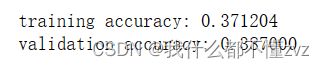
# Write the LinearSVM.predict function and evaluate the performance on both the
# training and validation set
y_train_pred = svm.predict(X_train)
print('training accuracy: %f' % (np.mean(y_train == y_train_pred), ))
y_val_pred = svm.predict(X_val)
print('validation accuracy: %f' % (np.mean(y_val == y_val_pred), ))
学习并更新参数
# Use the validation set to tune hyperparameters (regularization strength and
# learning rate). You should experiment with different ranges for the learning
# rates and regularization strengths; if you are careful you should be able to
# get a classification accuracy of about 0.39 (> 0.385) on the validation set.

# Note: you may see runtime/overflow warnings during hyper-parameter search.
# This may be caused by extreme values, and is not a bug.

# results is dictionary mapping tuples of the form
# (learning_rate, regularization_strength) to tuples of the form
# (training_accuracy, validation_accuracy). The accuracy is simply the fraction
# of data points that are correctly classified.
results = {}
best_val = -1   # The highest validation accuracy that we have seen so far.
best_svm = None # The LinearSVM object that achieved the highest validation rate.

################################################################################
# TODO:                                                                        #
# Write code that chooses the best hyperparameters by tuning on the validation #
# set. For each combination of hyperparameters, train a linear SVM on the      #
# training set, compute its accuracy on the training and validation sets, and  #
# store these numbers in the results dictionary. In addition, store the best   #
# validation accuracy in best_val and the LinearSVM object that achieves this  #
# accuracy in best_svm.                                                        #
#                                                                              #
# Hint: You should use a small value for num_iters as you develop your         #
# validation code so that the SVMs don't take much time to train; once you are #
# confident that your validation code works, you should rerun the validation   #
# code with a larger value for num_iters.                                      #
################################################################################

# Provided as a reference. You may or may not want to change these hyperparameters
learning_rates = [1e-7, 5e-5]
regularization_strengths = [2.5e4, 5e4]

# *****START OF YOUR CODE (DO NOT DELETE/MODIFY THIS LINE)*****

for lr in learning_rates:
    for rs in regularization_strengths:
        svm = LinearSVM()
        loss_hist = svm.train(X_train,y_train,learning_rate=lr,reg=rs,num_iters=1000,verbose=True)
        y_train_pred = svm.predict(X_train)
        y_val_pred= svm.predict(X_val)
        train_acc=np.mean(y_train == y_train_pred)
        val_acc=np.mean(y_val == y_val_pred)
        results[(lr,rs)]=train_acc,val_acc
        if(val_acc>best_val):
            best_svm=svm
            best_val=val_acc

# *****END OF YOUR CODE (DO NOT DELETE/MODIFY THIS LINE)*****

# Print out results.
for lr, reg in sorted(results):
    train_accuracy, val_accuracy = results[(lr, reg)]
    print('lr %e reg %e train accuracy: %f val accuracy: %f' % (
                lr, reg, train_accuracy, val_accuracy))

print('best validation accuracy achieved during cross-validation: %f' % best_val)
要点:
- 遍历learning_rate、regularization_strengths
- 创建SVM对象,调用svm.train函数
- 预测training set和validation set
- 返回精确度,如果精确度更好,保存当前的svm对象以及精确度
可视化学习率、正则系数、精确度
# Visualize the cross-validation results
import math
import pdb

# pdb.set_trace()

x_scatter = [math.log10(x[0]) for x in results]
y_scatter = [math.log10(x[1]) for x in results]

# plot training accuracy
marker_size = 100
colors = [results[x][0] for x in results]
plt.subplot(2, 1, 1)
plt.tight_layout(pad=3)
plt.scatter(x_scatter, y_scatter, marker_size, c=colors, cmap=plt.cm.coolwarm)
plt.colorbar()
plt.xlabel('log learning rate')
plt.ylabel('log regularization strength')
plt.title('CIFAR-10 training accuracy')

# plot validation accuracy
colors = [results[x][1] for x in results] # default size of markers is 20
plt.subplot(2, 1, 2)
plt.scatter(x_scatter, y_scatter, marker_size, c=colors, cmap=plt.cm.coolwarm)
plt.colorbar()
plt.xlabel('log learning rate')
plt.ylabel('log regularization strength')
plt.title('CIFAR-10 validation accuracy')
plt.show()

测试集预测
# Evaluate the best svm on test set
y_test_pred = best_svm.predict(X_test)
test_accuracy = np.mean(y_test == y_test_pred)
print('linear SVM on raw pixels final test set accuracy: %f' % test_accuracy)
![]()
可视化权重矩阵
# Visualize the learned weights for each class.
# Depending on your choice of learning rate and regularization strength, these may
# or may not be nice to look at.
w = best_svm.W[:-1,:] # strip out the bias
w = w.reshape(32, 32, 3, 10)
w_min, w_max = np.min(w), np.max(w)
classes = ['plane', 'car', 'bird', 'cat', 'deer', 'dog', 'frog', 'horse', 'ship', 'truck']
for i in range(10):
    plt.subplot(2, 5, i + 1)

    # Rescale the weights to be between 0 and 255
    wimg = 255.0 * (w[:, :, :, i].squeeze() - w_min) / (w_max - w_min)
    plt.imshow(wimg.astype('uint8'))
    plt.axis('off')
    plt.title(classes[i])
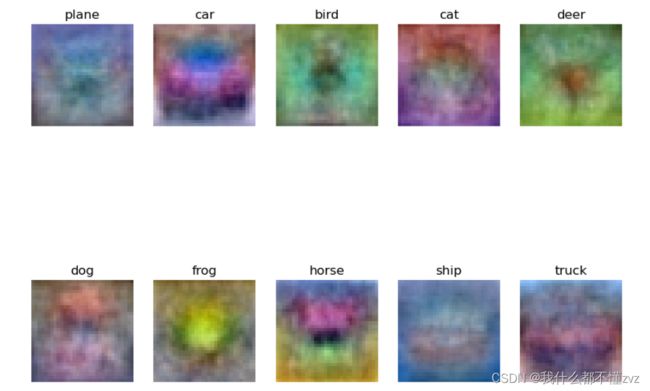
内嵌问题2:描述你看到的权重矩阵可视化的样子,为什么他们会这样?
因为提取的是所有同一类别训练照片的特征,比如horse,两个头,说明训练集的照片中马的照片有左边头和右边头的。