matlab连续投影算法SPA使用示例
连续投影算法(Successive Projections Algorithm,SPA)是一种使矢量空间共线性最小化的前向变量选择算法, 它的优势在于提取全波段的几个特征波长,能够消除原始光谱矩阵中冗余的信息,可用于光谱特征波长的筛选。
——百度百科
论文写作需要用到SPA对高光谱数据进行波段选择,在网上找到相关代码SPA_GUIhttp://www.ele.ita.br/~kawakami/spa/后不知道如何使用,于是参考帮助文档一步一步的做。以下内容来自帮助文档内第七章节示例。
链接:https://pan.baidu.com/s/1yoWpCvIneq5cfRxfZG8P5w
提取码:ylhl
SPA工具、帮助文档和示例数据都放在wangpan里了
前情提要
网上看的问题大多出在不知道Xcal、Ycal和Xval、Yval是什么东西,根据我的理解,Xcal、Ycal 分别是建模集的光谱反射率矩阵和待测物质含量(比如植株含水量、叶面积指数、生物量等等这些生理参数,我这里是拿农业方面做例子,还可以是其他学科的一些参数);Xval、Yval 分别是验证集或者叫预测集光谱反射率矩阵和待测物质含量。就是说,同一批光谱数据分析之前先要划分样本集,将所有样本划分为建模集和验证集。而且这些矩阵是行为样本,列为波段,也就是说第一行是样本1,这一行从第一列开始往后都是这个样本的反射率。
算法实现
1、数据设置
数据使用示例数据,获取数据代码如下(也是从网站http://www.ele.ita.br/~kawakami/spa/Extract_corn_dataset.m直接获取的):
原始数据放在wangpan里:链接:https://pan.baidu.com/s/1vdNrXhKgQlfGJM70jENOYQ
提取码:bz2t
urlwrite(['http://www.eigenvector.com/data/Corn/corn.mat'],'corn.mat'); % Extracts the corn data set from URL www.eigenvector.com
%%
warning('off')
load('corn.mat') % Loads the data set
warning('on')
data = [m5spec.data propvals.data(:,1)];% Arranges the data into a matrix: Samples x (Spectral variables + Moisture content)
clearvars -except data
save corn_dataset % Saves the dataset
delete('corn.mat') % Removes the temporary file
直接运行,运行时间很长慢慢等待就好,运行完毕后会出现corn_dataset.mat这个文件,打开可以看到,是一个80×701的一个矩阵,正如前情提要里说到,行为样本列为波段。根据帮助文档里所写,这个数据是80个玉米样本反射率数据1到700列,而且第701列数据为玉米含水量(The data set used in this example consists of spectra from 80 corn samples, which were acquired in the range 1100–1498 nm, together with moisture content for each sample.光谱范围是1100到1498但是为啥会有700个波段可能是帮助文档写错了吧)。

2、数据导入Loading the data
运行SPA_GUI.p文件,会出现下列界面,然后选择Load,把那个玉米数据集导入。
In the “Load Data” module (section 3) use the “load” button to load the contents of data file tothe workspace.Once the data file is loaded, the matrix “data” is presented at the “Data matrices in the workspace” group.
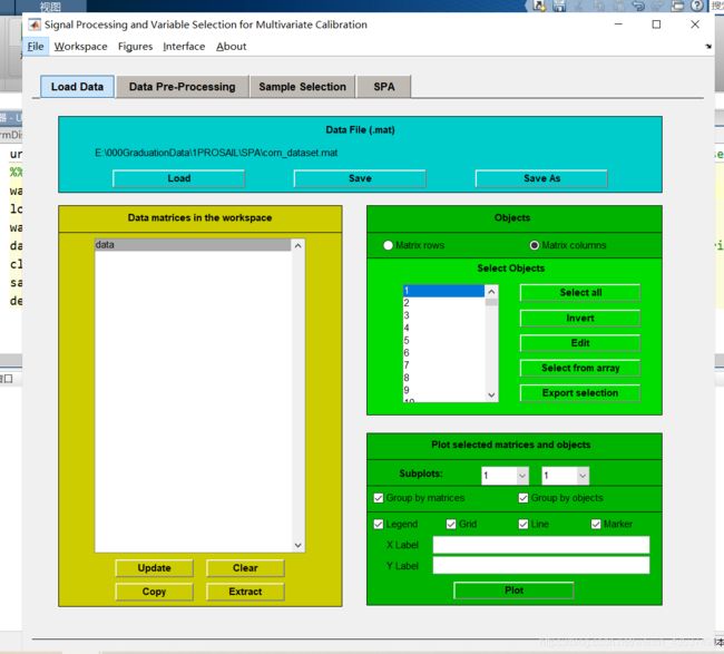
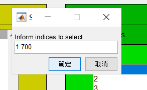
然后在Objects里选择Matrix Columns,意思是按列选择。然后点击Edit,输入1:700,点击确定就会选择前700列数据,点击Extract提取当作X(后续还要对X进行处理,处理得到Xcal、Xval)。
The next step is to split the data matrix will in the matrices X (instrumental responses) and Y (parameter of interesting). In order to do that, first select the “Matrix Columns” checkbox and press the “Edit” button in the “Objects” group. The following window will appear. In this window, select the columns with index of 1 to 700 and press the OK button.To extract the data to Y, repeat the process selecting only the column 701.


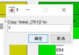
这个时候Data matrices in the workspace里就会出现提取的X。同样方法提取第701列数据玉米含水量当作Y(后续还要对Y进行处理,处理得到Ycal、Yval)。
3、数据预处理Preprocessing
这个示例使用了Savitzky–Golay一阶平滑消除光谱噪声,降低环境背景干扰等因素的影响。当然程序还提供了wavelet denoising小波去噪的处理方法。
This module contains the following groups: “Savitzky-Golay Smoothing”, “Savitzky-Golay Differentiation”, and “Wavelet Denoising”.
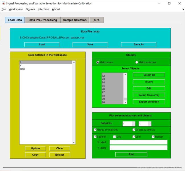
首先要先全部选择X中的数据。Objects里选择Matrix Rows,然后Select All。
To perform this preprocessing, select the matrix “X” in the “Data matrices in the workspace” group. Then, in the “Objects” group, select the “Matrix rows” option and press the button “Select All” to select all samples.
随后切换到Data Pre-Processing界面,设置S-G平滑的相关参数。
Switch to the “Data Pre-Processing” module. In this module, inform the Savitzky-Golay filter parameters (the frame size, polynomial order, and differentiation order), according to the figure below.
Frame Size一定是奇数,值越大,则平滑效果越明显。
Polynomnial设置平滑多项式的次数。通常设置为2~4。较低的次数能够产生平滑结果,但是有可能出现偏置。较高的次数能降低偏置,但有可能过拟合而导致结果噪声过多。次数必须小于滤波器宽度,即Frame Size。
Order设置导数阶数。设置为0,表示仅平滑;设置为1,表示一阶导数平滑结果;设置为2,表示二阶导数。以此类推(Order必须小于等于Polynomial)。
The frame size must be odd, and the polynomial order must be less than the frame length. If invalid parameters are entered, error messages will appear.
The same parameters specified for Savitzky-Golay smoothing will be also used for Savitzky- Golay differentiation. To run the differentiation, it is also necessary to specify the differentiation order (1 or 2, meaning first or second derivative).
然后Apply即可,会出现S-G平滑后的结果。
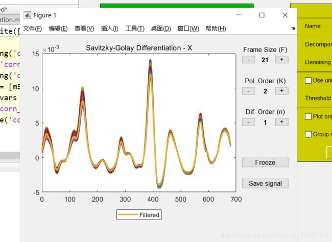
可以用+ -来修改S-G平滑的参数。
If want to test other preprocessing configurations, press the “+” and “-” buttons to change the frame size and polynomial order.
随后点击Save Signal来保存S-G平滑结果,结果保存为Xnew 。
Press the “Save signal” button in the Savitzky-Golay screen to save the processed samples. A window requesting the name of the matrix will appear. In this window, inform the name of the matrix as “Xnew”.
4、样本选择Selection of samples
这个示例使用了Kennard-Stone算法来选择样本。当然程序还提供了随机选择Random Sampling和SPXY算法。
把这80个样本分成40建模20验证20预测,切换到Sample Selection界面,参数设置如下图所示。
The KS algorithm is used to divide the available samples into calibration, validation, and prediction sets. The corn data were divided into 40 samples for calibration, 20 samples for validation, and 20 samples for prediction. These sets are used for model-building and performance evaluation.
To select the 40 samples for calibration, switch to the “Sample Selection” module and set the parameters as in the following figure.

点击run,便会对X和Y数据进行选择。
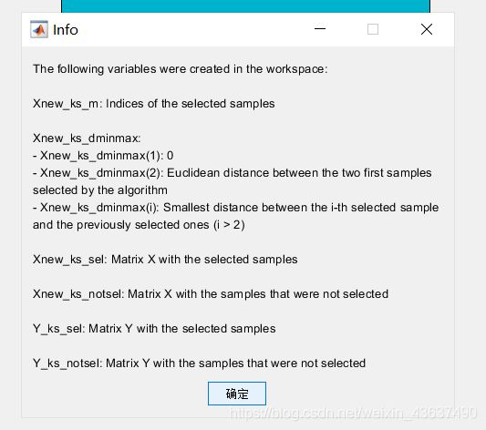
可以看到,Xnew_ks_sel包含被选择作为建模的样本,也就是Xcal,而Xnew_ks_notsel中是未被选中建模的样本,这个矩阵中包含验证和预测的样本所以要进一步拆分。Y_ks_sel就是Ycal
The “Xnew_ks_sel” matrix, which contains the selected samples, is the set to be used for calibration. The “Xnew_ks_notsel’ matrix, which contains the samples that were not selected, will be divided in two sets, for validation and prediction.
Before dividing the “Xnew_ks_notsel” matrix, it will first be ordered according with Euclidian distances using the KS algorithm. This procedure can be performed by setting the parameters as in the following figure.
对Xnew_ks_notsel进一步拆分,参数设置如下。(根据自己的需要来设置,如果需要预测集就进行拆分,如果不需要预测集直接开始运行SPA了,Xnew_ks_notsel就是Xval。)


虽然设置的还是40,而且Xnew_ks_notsel_ks_sel与Xnew_ks_notsel所含内容是一致的,但是新生成的Xnew_ks_notsel_ks_sel是按照欧氏距离进行排序的。为了对其进行选择,切换到Load Data界面,在Data matrices in the workspace界面中选择Xnew_ks_notsel_ks_sel。
The new matrix “Xnew_ks_notsel_ks_sel” contains the same samples of “Xnew_ks_notsel”, but ordered by distance. In order to split this matrix in the validation and prediction sets, switch to the “Load Data” module and select the “Xnew_ks_notsel_ks_sel” matrix in the “Data matrices in the workspace” group.
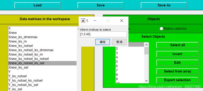
然后点击Edit,参数设置为1:2:40,意思是以2为间隔对数据进行选择。
Then, press the “Edit” button in the “Objects” group and select the samples 1:2:40, as illustrated in the figure below.
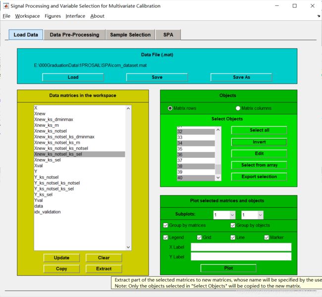
In order to extract the selected samples, press the “Extract” button in the “Data matrices in the workspace” group. The following window will appear. In this window, inform the name of the new matrix as “Xval” and press the OK button.

帮助文档中还写到,提取Xval后要将其导出以备后续之用。导出为idx_validation。(其实这个是为了保证后续Yval的选择是与Xval相对应的)
After that, press the “Export Selection” button in the “Objects” group to export the selected indices (for future use). The following window will appear. Inform the name of the array as “idx_validation”.
然后开始提取Yval。选择Y_ks_notsel_ks_sel,可以按照提取Xval的方法(就是设置1:2:40),也可以使用刚才导出的idx_validation。点击Select from array,并选择idx_validation,这样就会保证Xval与Yval是对应的(也就是一组反射率对应一个生理参数)。
Now, select the “Y_ks_notsel_ks_sel” matrix in the “Data matrices in the workspace” group to extract the moisture content for the validation samples.
The same indices used for matrix Xval must be used for matrix Yval. These indices can be informed by using the same procedure used above. An alternative procedure is to press the “Select from array” button in the “Objects” group. After pressing this button, a list of numeric matrices is presented. In this list, select the “idx_validation” array that was saved before. This will ensure that the same indices are used for Xval and Yval matrix.

选择预测数据集。先选择Xnew_ks_notsel_ks_sel,然后选择Select from array,再选idx_validation,再点击Invert就会反向选择,意思就是把Xnew_ks_notsel_ks_sel剩下的数据全选上。
To choose the samples of prediction, select the matrix Xnew_ks_notsel_ks_sel again in the “Data matrices in the workspace” group. Use the “Select from array” button to load again the list of indices available in the “idx_validation” array.
Press the “Invert” button in the “Objects” group to invert the selection, i.e., to select the remaining samples.
Now, set the matrix X for prediction using the “Extract” button in the “Data matrices in the workspace” group.
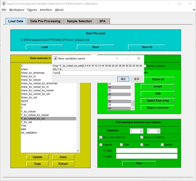
Select the matrix Y_ks_notsel_ks_sel in the “Data matrices in the workspace” group to extract the moisture content for the prediction samples.
Now, set the matrix Y for prediction using the “Extract” button in the “Data matrices in the workspace” group.
5、SPA算法运行Variable selection for multivariate calibration using SPA
5.1 建模
切换到SPA界面,把之前提取的Xcal等等参数设置一下,再设置筛选波段数量最大最小值即可。下图的参数都是按照帮助文档里的参数设置的,可以根据自己需要进行设置最大最小值。波段选择数据存储为var_sel。
To use the SPA algorithm, set the calibration and validation matrices, minimum and maximum number of variables as described in the section 6.1. In this example, specify the parameters as in the following figure and press the “Run SPA” button.
这个m_max一定小于样本数-1,但是也不一定非得设置为样本数-1,可以适当小一点这样才能选的多。有时候设置的大了SPA才选了1个波段出来。

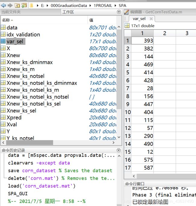
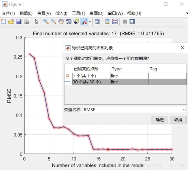
run之后会出现两个图,左边是误差分析图,右边是波段选择图。可以看到在第17次迭代时RMSE达到最小,于是选择了17个波段。波段选择的数据可以打开var_sel查看。
Two figures are presented: scree plot and the variables selected.
The scree plot tends to level off after a certain number of variables is added to the model. The number of variables selected in the third phase of SPA is indicated by square marker. This is the point at which the RMSE is not significantly larger than RMSEmin according to an F-test with a = 0.25.
The variables selected by SPA are plotted at the first calibration samples. This figure is presented below.

如果想保存RMSE这个图的数据,在RMSE这个figure里,点击刷亮/选择数据,然后全选数据,右键选择创建变量,保存RMSE数据即可。
5.2 样本预测
一般到SPA算法运行部分就可以了,样本预测这个部分我的论文里没有涉及,所以直接上帮助文档。
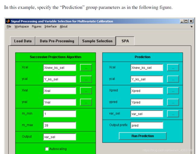
In this example, specify the “Prediction” group parameters as in the following figure.
The graph reference versus predicted is presented together with the statistics parameters PRESS, RMSEP, SDV, and r, for the prediction set. The figure below shows the obtained results.
To know the statistics parameter of the validation set, use the validation matrices in the spaces of prediction (Xpred and ypred). If they are left blank, leave-one-out cross-validation will be carried out in the calibration samples.
意思是如果Xpred和Ypred没有设置的话,会使用留一交叉验证法进行预测。

做完之后保存数据。
Switch to the “Load Data” module and press either the “Save” or the “Save As” button in the “Data File” group to save the data matrices to the data file (file with .mat extension).
In the main menu, choose the option “File: Save” or “File: Save As” to save the configuration file (file with .spr extension used to store the parameters specified in the graphical user interface).


