GNN-CS224W: 1-2 Introduction； Traditional Methods for machine learning in Graphs

network相比其他的数据有很多特点让它难以处理：

arbitrary size and complex topological structure

Applications of Graph ML

task level

Node-level

Predict a property of a node
Example: Categorize online users / items

Alpha Fold

task: Computationally predict a protein’s 3D structure based solely on its amino acid(氨基酸) sequence

Key idea: “Spatial graph” (represent the underlying protein as a graph)
Nodes: Amino acids in a protein sequence
Edges: Proximity between amino acids (residues) (在空间中接近的node之间构建边)

模型：给定Amino acids的位置及edges proximities between them 然后预测新的Amino acids的位置（还是 Amino acids的新位置），从而最终预测amino acids的位置和protein的最终形态

Edge-level

Predict whether there are missing links between two nodes
Example: Knowledge graph completion

Recommender system

Node: users, items(songs, merchandise…)
Edge: user-item interactions
Goal: recommend items user might like

Drug side effects–Biomedical graph link prediction

有的人可能会吃多种药，目的是预测不同种类的药物同时服用时的副作用
药物太多，导致不可能对所有药物组合试验其副作用，所以采用机器学习来预测

Task: Given a pair of drugs predict adverse side effects
Nodes: Drugs & Proteins
Edges: Interactions between drugs and proteins, Interactions between proteins, Interactions between drugs (drugs之间的interaction代表adverse side effects)
node之间的edge有的是知道的，用模型来预测missing edges

Community (subgraph) level

Detect if nodes form a community(团体)
Example: Social circle detection
相当于cluster，找出社交网络中联系紧密的小团体

Traffic prediction

road network as a graph
Node: Road segments
Edge: connection between road segments
task: 给出从一个node到另一个node的路线

Graph-level

Categorize different graphs
Example: Molecule property prediction

Drug discover

Antibiotics(抗生素) are small molecular graphs
Nodes: Atoms
Edges: Chemical bonds(化学键)
Task: 预测一个分子是否有能被当做药物

原子组合成的分子太多了，无法做到所有的都做药物试验，所以需要机器学习来预测更有可能有用的分子

Graph generation – Drug discovery

还是将原子作为node，化学键作为edges
User case 1: Generate novel molecules with high drug likeness
Use case 2: Optimize existing molecules to have desirable properties (把已有的分子碎片扩展成有特定作用的大分子)

Graph evolution – Physical simulation

Physical simulation as a graph
Nodes: Particles
Edges: Interaction between particles
Task: 预测这些particles将来的状态

Choice of graph representation, how do we define a graph?

the choice of what the nodes are and what the links are are very important.

同样的数据可以选择很多不同的对象作为node和link，node和link的选择对模型效果很重要

Objects: nodes, vertices N
Interactions: links, edges E
System: network, graph G(N,E)

Directed and Undirected Graph

Undirected Graph

node之间的关系是 symmetrical(对称的), reciprocal(相互的)

Examples: Collaborations, Friendship on Facebook

Directed Graph

every link has a direction, a source, a destination
Examples: Phone calls, Following on Twitter

Node degrees

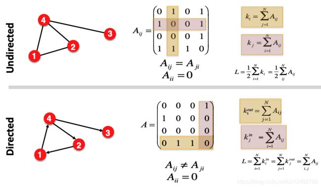
Node degree: $k_i$ the number of edges adjacent to node i, (包括入度和出度)例如$k_i=4$
Average degree: $\frac{1}{N}\sum _{i=1}^N{k}_i=\frac{2E}{N}$

directed graph node has In degree and Out degree

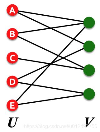
Bipartite graph

如图所示，满足如下特性：

1. all nodes can be divided into two disjoint(不相交) set U and V
2. every link connects a node in U to one in V
3. U and V are independent set

Examples:
§ Authors-to-Papers (they authored)
§ Actors-to-Movies (they appeared in)

Folded/Projected Bipartite graph

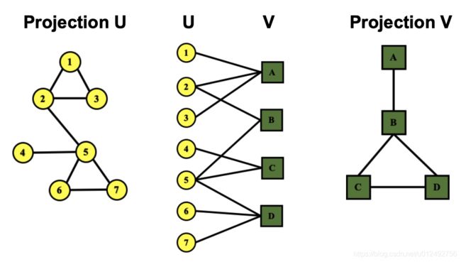
如上图所示，Bipartite graph可以将一边fold起来，fold后graph中的边表示两个node是否可以通过另一边的node连通
假设上图中表示的是author和paper的关系，左边黄点表示author，右边方块便是paper，则根据没有fold的bipartite graph可知，1 2 3三位作者合作了paper A，则1 2 3在fold后的图里是连通的，2和5合作了paper B，则2和5在fold后的图里是连通的。另一边也可以用同样的逻辑fold起来。

Representing graphs

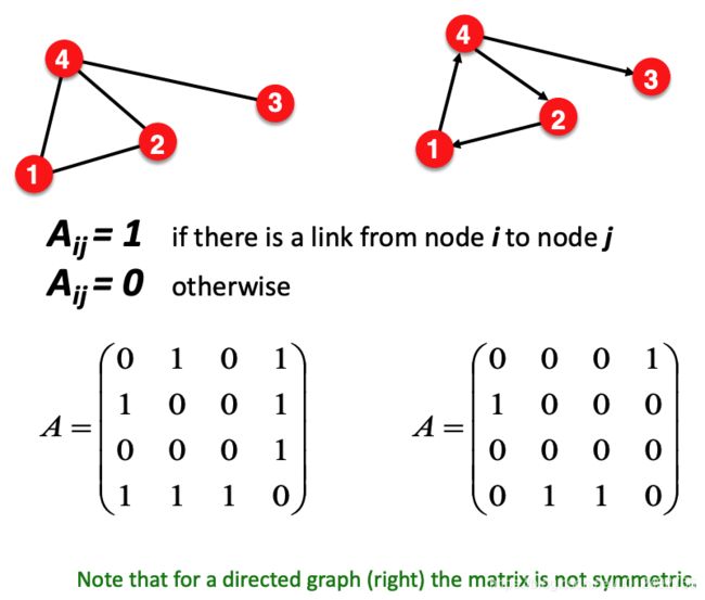
Adjacent matrix

Most real-world networks are sparse, 这导致了 Adjacent matrix 也sparse
例如人们的社交网络，世界上一共有70亿人，但是一个人只能跟很少一部分建立关系，剩余大量的人都没有关系

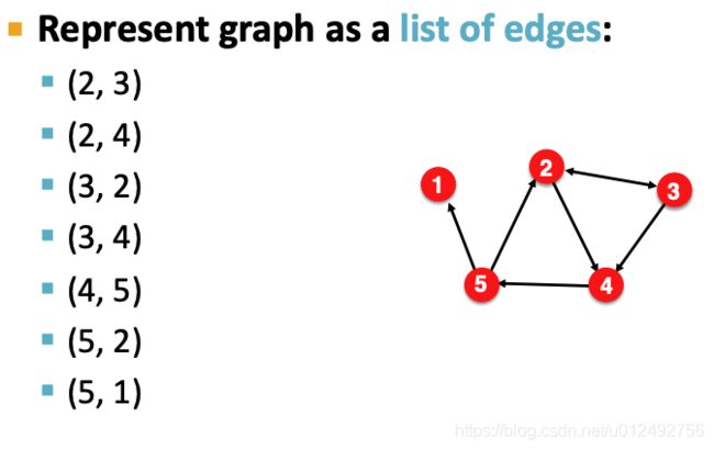
Edge list

将graph表示为一个二维的matrix

缺点是不能做任何graph manipulation和analysis of the graph

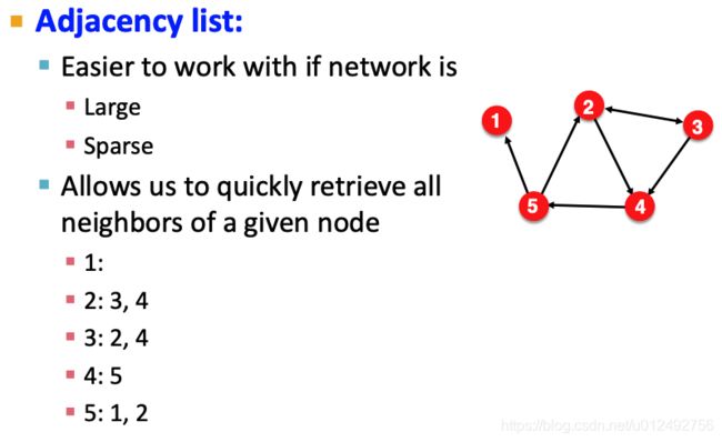
Adjacency list

优点：

1. 支持 graph manipulation和analysis of the graph
2. 相比adjacent matrix存储空间大大减少
   可以二维矩阵来存储，因为边很少，所以列数会较小

Node, edge and graph attributes

Possible options:

1. Weight (e.g., frequency of communication)
   weight可以直接体现在adjacent matrix上
2. Ranking (best friend, second best friend…)
3. Type (friend, relative, co-worker)
4. Sign: Friend vs. Foe, Trust vs. Distrust
5. Properties depending on the structure of the rest of the graph: Number of common friends

more types of graphs

1. self-edges
   节点有从自己出发、指向自己的边，体现在adjacent matrix上就是对角线元素为1
2. multigraph
   两个节点之间不只有一条边。有时边含义相同，则可以边的数量可以认为是weight；有时边含义不同，不能认为是weight。

连通图和非连通图

Undirected

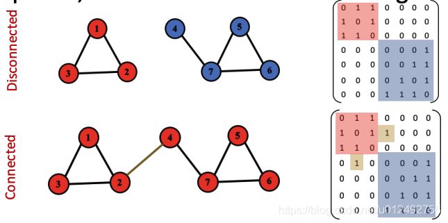
连通图和非连通图的差别可以提现在adjacent matrix，如下图

Directed

1. Strongly connected directed graph (强连通图)
   has a path from each node to every other node and vice versa (e.g., A-B path and B-A path)
2. Weakly connected directed graph (弱连通图)
   is connected if we disregard the edge directions

Strongly connected components (SCCs) (强连通分量)

Traditional Methods for machine learning in Graphs

Traditional ML pipeline

1. Design features for nodes/links/graphs
   node feature: 例如 protein attributes
   例如node在整个network里处于什么位置，node附近的结构是怎样的

   特征可以被分为2种：

   1. network structure
   2. nodes/links/graphs properties

2. Obtain features for all training data

Node-level tasks and features

Goal: Characterize the structure and position of a node in the network，通常有如下4种特征：

Node degree

Node degree counts the neighboring nodes without capturing their importance.

Node centrality

Node centrality(中心)表示一个node是不是graph的中心，是中心的程度是多少

有如下几种方式

Engienvector(特征向量) centrality

A node $v$ is important if surrounded by important neighboring nodes $u\in N(v)$.

node $v$的centrality的计算方式：

$$c_v=\frac{1}{\lambda }\sum _{u\in N(v)}{c}_u$$

其中$\lambda$是一个正的常数，称为eigenvalue(特征值)。上式可以写成matrix form：

$$\lambda c=Ac$$

其中A为adjacent matrix, c称为为eigenvector

问题

1. The largest eigenvalue ${\lambda }_{max}$ is always positive and unique (by Perron-Frobenius Theorem). The leading eigenvector $c_{max}$ is used for centrality
2. 每个节点的重要性都取决于周围的节点，是否最开始有一些节点被指定了重要性？要不然都依赖于周围，那一步一步往外推，最外层的节点依赖谁？

Betweenness centrality

Intuition: A node is important if it lies on many shortest paths between other nodes
$$c_v=\sum _{s\ne v\ne t}\frac{\#(shortestpathsbetwensandtthatcontainv)}{\#(shortestpathsbetweensandt)}$$

"#"表示the number of

Closeness centrality

Intuition: A node is important if it has small shortest path lengths to all other nodes.

$$c_v=\frac{1}{\sum _{u\ne v}shortestpathlengthbetweenuandv}$$

and many others…

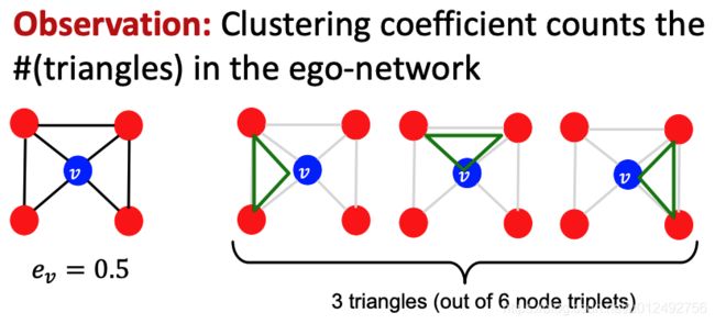
Clustering coefficient

Intuition: Measures how connected neighboring nodes are。即一个node的 neighbor 之间的联系是否紧密

$$e_v=\frac{\#(edgesamongneighboringnodes)}{C_{k_v}^2}$$

其中分子表示node v的neighbor node之间实际的edge数量；$k_v$表示node v的degree，分母表示从node v的neighbor node中挑选2个时一共有多少种情况，即node v的neighbor node一共有多少个可能的edge

Another view

Graphlets

we can generalize the above (counting #(trangles) ) by counting #(pre-specified subgraphs, i.e., graphlets).

什么是graphlet

如下图为包括2个到5个node的graphlets
isomorphic(同构)

要注意的是每个graphlet中部分节点被标注了数字，被标数字的node表示当前要得到的是这个node的特征，也就是让该node处于图中的位置的graphlet；数字的大小表示这是第多少种情况，例如3个节点的graphlets一共有2个图，但是有3个graphlet，G2中每个位置都是等价的，所以只有一个graphlet，G1中从位置1和位置2的角度看，G1代表的图是不同的，所以有2个graphlet

Graphlet Degree Vector (GDV)

GDV如下图所示，一个node对应一个向量，向量的每个维度对应一种graphlet，数字表示该graphlet的数量

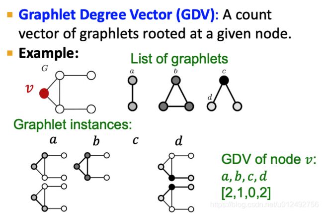
Considering graphlets on 2 to 5 nodes we get: Vector of 73 coordinates is a signature of a node that describes the topology of node’s neighborhood, Captures its interconnectivities out to a distance of 4 hops(5个node的结构需要4条边)

作用

作用：Graphlet degree vector provides a measure of a node’s local network topology

Comparing vectors of two nodes provides a more detailed measure of local topological similarity than node degrees or clustering coefficient.

Node features 分类总结

Importance-based features

capture the importance of a node is in a graph

1. Node degree
2. Different node centrality measures

Useful for predicting influential nodes in a graph，Example: predicting celebrity(名人) users in a social network

Structure-based features

Capture topological properties of local neighborhood around a node

1. Node degree
2. Clustering coefficient
3. Graphlet count vector

Useful for predicting a particular role a node plays in a graph: Example: Predicting protein functionality in a protein-protein interaction network.

Link-level prediction tasks and features

Task: predict new links based on existing links.

方式：all node pairs (no existing links, 所有以前不存在的link) are ranked, and top k node pairs are predicted

Key: design features for a pair of nodes.

只用node feature的话将会缺少link信息

Two formulations of the link prediction task

Links missing at random:

Remove a random set of links and then aim to predict them

更适合static network，例如protein-protein network

Links over time

这种task假设有一个不断变化的network，例如social network、citation network

Given $G[t_0,t_0^{\prime }]$ (a graph on edges up to time $t_0^{\prime }$, ), output a ranked list L of links (not in $G[t_0,t_0^{\prime }]$) that are predicted to appear in $G[t_1,t_1^{\prime }]$

Evaluation 方式：在实际环境中得到 new edges that appear during the test period [t_1,t_1’]，和预测的edges做比较

只适用于dynamic network，例如protein-protein network

问题：这里没说清楚$t_0,t_0^{\prime }$的关系，$G[t_0,t_0^{\prime }]$是一个时间序列及其对应的graph吗？还是只是一个时间点的graph？为什么预测的link不能在$G[t_0,t_0^{\prime }]$里？

Methodology 常见步骤

1. For each pair of nodes (x,y) compute score c(x,y)
   For example, c(x,y) could be the number of common neighbors of x and y
2. Sort pairs (x,y) by the decreasing score c(x,y)
3. Predict top n pairs as new links
4. See which of these links actually appear in $G[t_1,t_1^{\prime }]$

Link-level features

Goal: give two nodes, describe the relationship between them, then predict or learn whether there exists a link between them

Distance-based feature

Local neighborhood overlap feature

Captures number of neighboring nodes shared between two nodes $v_1$ and $v_2$:

Adamic-Adar index中，如果一个node的degree($k_u$)很大 =>$\log k_u$较大 => $\frac{1}{\log k_u}$较小
这意味着两个node的共同neighbor中，degree大的发挥的作用小，degree小的发挥的作用大

例如social network中，如果两个人都是同一个明星的粉丝，不意味着两个人之间存在什么关系，但是如果两个人都是一个粉丝数量很少的人的粉丝，则这两个人有关系的可能性更大

缺点：Metric is always zero if the two nodes do not have any neighbors in common.However, the two nodes may still potentially be connected in the future.例如下图所示的情况

这里的local(局部)的意思是只考虑了$v_1$ and $v_2$的neighbor，而network里其他的node没有被考虑

Global neighborhood overlap feature

相比Local neighborhood overlap feature，考虑了 the entire graph

一种Global neighborhood overlap feature：
Katz index: count the number of paths of all lengths between a given pair of nodes

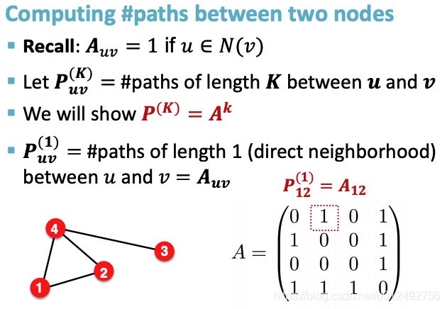
Use powers of the graph adjacency matrix to compute the number of paths for a give length between two nodes

powers of the graph adjacency matrix

$A^{(k)}$中，k(幂的次数)代表了当前矩阵里的path的length
若$A_{uv}^{(k)}\ne 0$，则u和v之间存在长度为k的path，path数量为$A_{uv}^{(k)}$

现在继续看Katz index

Katz index between $v_1$ and $v_2$ is calculated as sum over all path lengths
$$S_{v_1{v}_2}=\sum _{l=1}^{\infty }{\beta }^l{A}_{v_1{v}_2}^l$$

其中$0<\beta <1$，为discount factor。式子的意思是$v_1$ and $v_2$之间越短的path的权重越大，越远的path的权重越小。 $S_{v_1{v}_2}$越大，表示两个节点联系越紧密。

Katz index matrix is computed in closed-form:
$$S=\sum _{i=1}^{\infty }{\beta }^i{A}^i=(I-\beta A{)}^{-1}-I$$

计算是根据 geometric series of matrices (矩阵的几何级数) 计算得出的, $(I-\beta A{)}^{-1}=\sum _{i=0}^{\infty }{\beta }^i{A}^i$,

Graph-level features and graph kernals

Kernel methods

widely-used for traditional ML for graph-level prediction

Idea: Design kernels instead of feature vectors
普通方法为先对graph提取特征形成特征向量，把特征向量作为模型输入；Kernel methods 也要先对graph提取特征形成特征向量，但是两个graph的特征向量求dot可以直接得到相似度，无需再对特征向量建模

Kernel $K(G,G^{\prime })\in R$ measures similarity between data

Kernal matrix $\text{K}=(K(G,G^{\prime }){)}_{G,G^{\prime }}$, must always be positive semidefinite (i.e., has positive eigenvals)

There exists a feature representation $\varphi (\cdot )$ such that $K(G,G^{\prime })=\varphi (G{)}^T\varphi (G^{\prime })$

Once the kernel is defined, off-the-shelf ML model, such as kernel SVM, can be used to make predictions.

问题：

1. 什么是positive semidefinite matrix(半正定矩阵)？
2. 为什么要存在$\varphi (\cdot )$？有什么意义？

Graph-level features: Graph kernals

Goal: Design features that characterize the structure of an entire graph to compute similarity

Graph kernal: Key Idea

这里是Graph kernal 方法的一个简单例子

1. 特征1：Bag-of-Words (BoW) for a graph

   类似表示文本的Bag-of-Words，用一个特征向量表示graph，向量长度为所有graph可能的node总数量，其中每个值表示对应的node在具体一个graph中是否出现

   这种方法能包含的信息量非常有限，会让很多结构不同的图得到相同的表示，例如下图
   
   其中$\varphi$表示graph的特征向量

2. 特征2：Bag of node degrees

   使用node degrees生成特征向量，包含的信息比特征1更多，如下图所示：
   

这里的特征1和特征2都是比较初级的Graph kernal方法，下面两个是更高级的方法

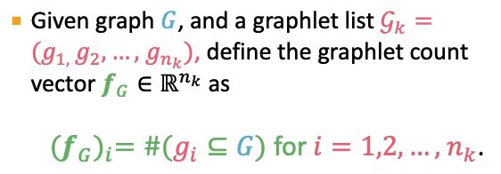
Graphlet Kernel

Key idea: Count the number of different graphlets in a graph.

Definition of graphlets here is slightly different from node-level features.

1. Nodes in graphlets here do not need to be connected (allows for isolated nodes)
2. The graphlets here are not rooted.

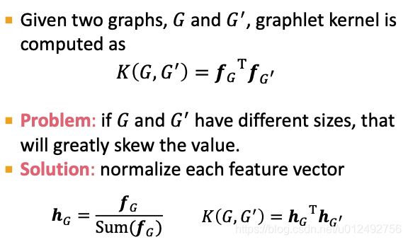
其中$Sum(f_G)$表示对特征向量的所有值求和，例如上面例子中$f_G=(1,3,6,0{)}^T$求sum等于10

Limitations

Counting graphlets is expensive!

Weisfeiler-Lehman Kernel

more computing efficient than Graphlet Kernel

Idea: use neighborhood structure to iteratively enrich node vocabulary

实现方法：Color refinement

Color refinement

算法描述：

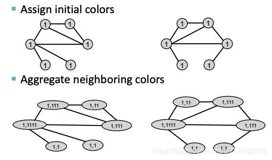
例子：如下图所示，用1代表初始的color，第一步将node的neighbor都添加到node里，第二步将node和neighbor的组合信息用一个hash 函数映射到另一个color上。这两步就是一次aggregate操作，此时每个节点的颜色包含了node自己的信息以及直接neighbor的信息


如下图所示进行第二次aggregate操作，对此时的node来说，它已经包括了它的直接neighbor信息，aggregate结束后每个node就包括了距离node 2 步的间接neighbor信息

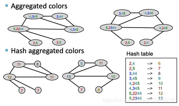
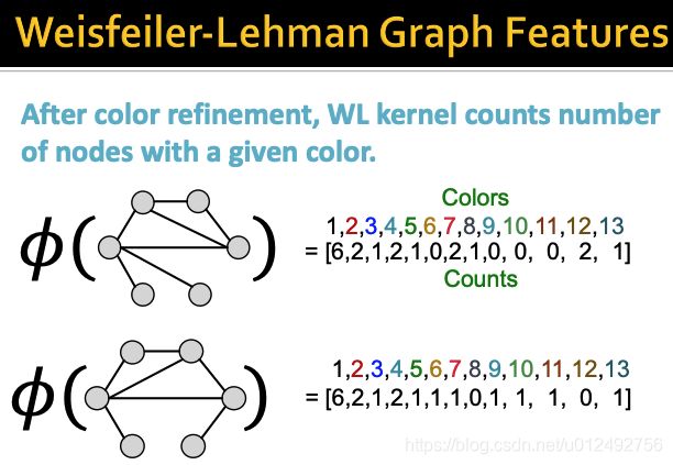
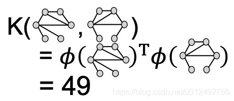
理解

可以有效的集合大量的各种距离的neighbor信息

第一步操作时集合将了距离节点为1的节点的信息，第二步时集合了距离节点为2的节点的信息，第K步后，每个节点就包含所有距离它K的节点的信息

time complexity

1. at each step the time complexity is linear in #(edges) (the number of edges)
2. #(colors) is at most the total number of nodes
   color是可以复用的，只要每一步的color是彼此独立的即可，所以最多只需要节点数量个color
3. Counting colors takes linear-time w.r.t. #(nodes).
   这一步是最后形成feature vector时对每一种颜色计数，只需要#(nodes)次计算

In total, time complexity is linear in #(edges).

Other kernels

(beyond the scope of this lecture)

1. Random-walk kernel
2. Shortest-path graph kernel
   And many more…