Sklearn XGBoost模型算法分类建模-----风控项目实战（PR曲线、KS、AUC、F1-Score各类指标）

项目背景:二手手机需从前端质检项推断手机有无拆修问题
思路：
a)X值:前端各类质检项，对应映射ID+RANK值(涉及质检项会有等级排序，需进行RANK排序（属性值RANK一般需手工或是系统配置时候就有对应映射，如果是按照ID大小排序，则可以考虑SQL的进行rank() over(partition by))
b)Y值:业务角度选出有问题的手机质检项，拆修、进水等等，此类问题涉及到 多个属性值+多个属性值等级，需进行多层逻辑判断整合成 1，0，从而进行分类判断

代码逻辑:
a)读取数据，涉及数据较大且需pivot转换，这里考虑用yield进行分批读取

import numpy as np
import pandas as pd
# =============================================================================
# 数据清洗
# =============================================================================
property_value=pd.read_excel(r'C:\Users\116815\Desktop\建模属性项定义样本.xlsx',sheet_name='values')
property_value_merge=pd.read_excel(r'C:\Users\116815\Desktop\建模属性项定义样本.xlsx',sheet_name='values_merge')
num=36 #数据量
#读取数据
def yield_data(num):
    for num in range(1,num,1):
        data= pd.read_csv(r'D:\pycode\数据建模\建模数据\inspection_report_'+str(num)+'.csv')
        data.drop('inspection_dt',axis=1,inplace=True)
        data.drop_duplicates(inplace=True)
        data.dropna(inplace=True)
        data.drop(data[data['new_inspection_value_id']=='(NULL)'].index.values,axis=0,inplace=True)
        data['inspection_property_id']=data['inspection_property_id'].astype(int)
        data['new_inspection_value_id']=data['new_inspection_value_id'].astype(int)
        data=data.merge(property_value_merge,on=['new_inspection_value_id','inspection_property_id'],how='left')
        data_rank=data.pivot(index=['product_no'],columns=['inspection_property_id'],values='property_value_rank')  
        data=data.pivot(index=['product_no'],columns=['inspection_property_id'],values='new_inspection_value_id')  
        #data=data.applymap((lambda x: "".join(x.split()) if type(x) is str else x)) 
        yield data,data_rank
        

#迭代器分批处理数据
yield_data=yield_data(num)
data_list=[]
data_rank_list=[]
for i in range(1,num,1):
    data=next(yield_data)
    data_list.append(data[0])
    data_rank_list.append(data[1])
data=pd.concat(data_list)
data_rank=pd.concat(data_rank_list)

b)读取数据后，进行好坏样本转换，且根据专家经验剔除部分可能存在影响且排序较乱的属性ID

#好坏样本定义
data['good_bad']=1
for i in range(0,len(data),1):
    for j in [332,353,1279,2097,2098,2118]:
        #不为属性不检测和无异常，且不为空值
        if all(data[j].iloc[i] != x  for x in [2067,2129,6982,13791,13787,14165,12451,12453,12452,13794,13790,14168]) and pd.isnull(data[j].iloc[i])==False  :
            data['good_bad'].iloc[i]=0  
#删除坏样本判断属性项
data.drop([332,353,1279,2097,2098,2118],axis=1,inplace=True)
data_rank.drop([332,353,1279,2097,2098,2118],axis=1,inplace=True)
data.drop([456,806],axis=1,inplace=True)#去除颜色,内存
data_rank.drop([456,806],axis=1,inplace=True)#去除颜色,内存
#rank明细获取好坏属性
data_rank['good_bad']=data['good_bad']

c)模型选择，网格搜索最优参数(交叉验证)

# =============================================================================
# XGBOOST 可以考虑多模型 交叉验证后再去选模型 此处直接XGBOOST 出于此模型收敛快 且有缺失值
# =============================================================================
from xgboost import XGBClassifier,plot_importance
from sklearn.model_selection import train_test_split,GridSearchCV
from sklearn.metrics import roc_auc_score,roc_curve,precision_recall_curve
import matplotlib.pyplot as plt
import mglearn
# =============================================================================
#  训练 测试集
# =============================================================================
X=data_rank.iloc[:,:data_rank.shape[1]-2]
y=data_rank.iloc[:,data_rank.shape[1]-1]
X_train,X_test,y_train,y_test = train_test_split(X,y,test_size=0.2,random_state=10000)
# =============================================================================
# 网格搜索参数最优解
# =============================================================================
# param_grid = {
# 'max_depth':[i for i in range(3,12,2)],
# 'min_child_weight':[i for i in range(1,10,2)]
# }

# grid_search=GridSearchCV( estimator=(XGBClassifier(missing=0)), param_grid=param_grid,cv=5)
# grid_search.fit(X_train, y_train)
# print('best_params_',grid_search.best_params_)
# print('best_score_', grid_search.best_score_)
# print('best_estimator_',grid_search.best_estimator_)
# print("Test set score: {:.5f}".format(grid_search.score(X_test, y_test)))

# #交叉验证结果集
# results = pd.DataFrame(grid_search.cv_results_)
# scores = np.array(results.mean_test_score).reshape(5, 5)
# # 对交叉验证平均分数作图
# mglearn.tools.heatmap(scores, xlabel='max_depth', xticklabels=param_grid['max_depth'],
#  ylabel='min_child_weight', yticklabels=param_grid['min_child_weight'], cmap="viridis")

# =============================================================================
# 选出最优参数后 模型预测
# =============================================================================

xgbc = XGBClassifier(missing=0,max_depth=5,min_child_weight=9)
xgbc.fit(X_train, y_train)
print("Train set score: {:.5f}".format(xgbc.score(X_train,y_train)))
print("Test set score: {:.5f}".format(xgbc.score(X_test,y_test)))

y_test=y_test.values #转array
prdict_result=xgbc.predict(X_test)

d)相关指标(重要属性图、查全率、查准率、F1-SCORE、PR曲线、AUC绘图、KS值)

# =============================================================================
# TP FP FN TN
# =============================================================================
TP=0
FP=0
FN=0
TN=0
for i in range(0,len(y_test),1):
    if prdict_result[i]==y_test[i] and y_test[i]==1 :
        TP=TP+1
    elif prdict_result[i]==y_test[i] and y_test[i]==0:
        TN=TN+1
    elif prdict_result[i]!=y_test[i] and y_test[i]==1:
        FP=FP+1
    elif prdict_result[i]!=y_test[i] and y_test[i]==0:
        FN=FN+1
TPR=TP/(TP+FN)#正例预测
FNR=FN/(TP+FN)#正例预测为反例
TNR=TN/(FP+TN)#反例预测
FPR=FP/(FP+TN)#反例预测为正例
print(TP,TN,FP,FN)
print(TPR,FNR,TNR,FPR)

# =============================================================================
# 显示plt中文
# =============================================================================
from pylab import *
mpl.rcParams['font.sans-serif'] = ['SimHei']#中文字体
mpl.rcParams['axes.unicode_minus'] = False

# =============================================================================
# PR曲线 precision=TP/(FP+TP)  recall=TP/(TP+FN)
# =============================================================================
y_score = xgbc.predict_proba(X_test)
precision, recall, thresholds = precision_recall_curve(y_test, y_score[:,1])
balance_line=[]
for i in range(len(recall),0,-1):
        balance_line.append(1/i)
        
pd.DataFrame(precision*100)
plt.figure("P-R Curve")
plt.title('Precision/Recall Curve')
plt.xlabel('Recall')
plt.ylabel('Precision')
plt.plot(recall,precision,label='PR曲线')

plt.plot(balance_line,balance_line,linestyle='--',label='取值线')
plt.legend()
plt.show()

# =============================================================================
# 查全率（覆盖率）、查准率（命中率）和 F1score
# =============================================================================
i=0
k_percent=[]
for i in range(1,recall.shape[0]+1,1):
    k_percent.append(100*i/recall.shape[0])
    i=i+1
    
plt.xlabel('TOP K% OF THE SAMPLE')
plt.ylabel('%')
plt.plot(k_percent,precision,label='precision')
plt.plot(k_percent,recall,label='recall')
plt.legend()
plt.show()

####输出recall_precison_f1score_topn_topk数据
data_out=pd.DataFrame(recall*100).astype(int)
data_out.rename(columns={0:'recall(%)'},inplace=True)
data_out['precision(%)']=pd.DataFrame(precision*100).astype(int)
data_out.reset_index(inplace=True)
data_out['index']=data_out['index']+1
data_out['TOP K(%)']=round(100*data_out['index']/data_out.shape[0],2)
data_out.rename(columns={'index':'TOP N'},inplace=True)
data_out=data_out.groupby(['precision(%)','recall(%)']).max()
data_out.reset_index(inplace=True)
data_out_new=pd.DataFrame(data_out['precision(%)'])
data_out_new['recall(%)']=pd.DataFrame(data_out['recall(%)'])
data_out_new=data_out_new.groupby(['precision(%)']).min()
data_out_new.reset_index(inplace=True)
data_out=data_out_new.merge(data_out,on=['precision(%)','recall(%)'],how='left')


data_out['F1_score']=round(2*data_out['precision(%)']*data_out['recall(%)']/(data_out['precision(%)']+data_out['recall(%)']),2)
data_out.insert(2,'F1 score',data_out['F1_score'])
data_out.drop('F1_score',axis=1,inplace=True)

data_out.to_excel(r'D:\pycode\数据建模\recall_precision.xlsx')

# =============================================================================
# importance_features绘图
# =============================================================================

fig,ax = plt.subplots(figsize=(15,15))
plot_importance(xgbc,ax=ax,max_num_features=50)
plt.show()

# =============================================================================
# AUC绘图
# =============================================================================

#print("AUC:{:.5f}".format(roc_auc_score(y_test, xgbc.predict(X_test))))
fpr, tpr, thresholds= roc_curve(y_test, xgbc.predict_proba(X_test)[:, 1])
plt.plot(fpr,tpr, label="ROC Curve xgboost-{:.3f}".format(roc_auc_score(y_test, xgbc.predict(X_test))))
plt.xlabel('FPR')
plt.ylabel('TPR(RECALL)')
plt.title('AUC')
plt.legend()
plt.show()

# =============================================================================
# KS值
# =============================================================================
KS_point=0
for i in range(0,len(fpr),1):
    if tpr[i]-fpr[i]==max(tpr-fpr):
        KS_point=i
array_x=np.array([range(0,len(tpr) ,1)]).reshape(len(tpr),)
array_x_percent=array_x/len(array_x)
plt.plot(array_x_percent,tpr, label="good")
plt.plot(array_x_percent,fpr, label="bad")
plt.plot(array_x_percent,tpr-fpr, label='diff', linewidth=2)

plt.plot([array_x_percent[KS_point],array_x_percent[KS_point]], [tpr[KS_point],fpr[KS_point]], label='ks - {:.3f}'.format(max(tpr-fpr)), color='r', marker='o', markerfacecolor='r', markersize=5)
plt.legend()

print(max(tpr-fpr))
print(array_x_percent[KS_point])
# =============================================================================
# 导出模型
# =============================================================================
# dump it to a text file
xgbc.get_booster().dump_model(r'D:\pycode\数据建模\model\xgb_model.txt', with_stats=True)
## read the contents of the file
with open(r'D:\pycode\数据建模\model\xgb_model.txt', 'r',encoding='utf-8') as f:
     txt_model = f.read()
# print(txt_model)

# =============================================================================
#  XGBOOST可视化
# =============================================================================
import xgboost as xgb

digraph = xgb.to_graphviz(xgbc)
# 如果没有ipython的jupyter notebook，可以把此图写到pdf文件里，在pdf文件里查看。
digraph.format = 'png'
digraph.view(r'D:\pycode\数据建模\model\Xgboost')

##属性leaf是预测值
##分类情况下
#1/(1+np.exp(-1*(Leaf值相加))) 
##输出是指，先看各个样本在所有树中属于哪个节点，然后将各个树中的节点的值累加起来，然后还要乘以学习率才是输出，即叶子节点权重累加值乘以学习率。然后看objective是分类还是回归，如果是logistic，则求sigmoid即为概率值
##如果是logistic，则求sigmoid即为概率值

以上代码拼接，即为整体项目代码，项目整体来看模型还存在调优空间，且目前数据源为手机整体数据，后续可以考虑从IOS和ANDROID先进行区分，对其分别建模
具体图示如下：

a)最优参数网格搜索
采用5折验证(考虑性能暂未做特殊交叉验证)：

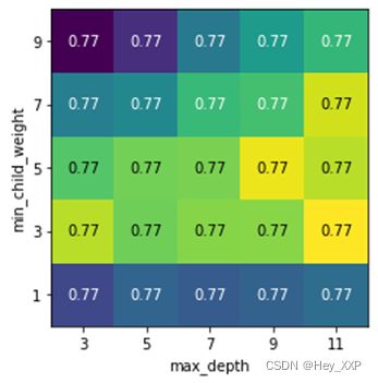
结论：参数选择存在问题，暂未对模型优化产生较大影响，后期优化(XGBOOST调优较难，会偏于稳定)

b)模型重要特征值
选用上述参数最优解，输出模型重要特征值(剔除了内存、颜色属性,俩类属性存在较高得分)：

c)相关指标
考虑数据总量11万，不做验证集拆解
训练集score：0.77913，测试集score：0.77019
AUC得分0.731
Type Score
训练集 0.77913
测试集 0.77019
AUC 0.731
KS 0.496

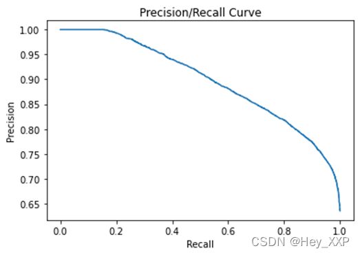
d)查准率、查全率、F1-SCORE

precision(%) recall(%) F1 score TOP N TOP K(%)
63 99 77 156 1.33
64 99 77.74 494 4.22
65 99 78.48 822 7.02
66 99 79.2 1152 9.84
67 99 79.92 1484 12.67
68 98 80.29 1826 15.59
69 98 80.98 2159 18.44
70 97 81.32 2500 21.35
71 97 81.99 2879 24.58
72 96 82.29 3261 27.85
73 94 82.18 3641 31.09
74 93 82.42 4019 34.32
75 91 82.23 4368 37.3
76 90 82.41 4726 40.36
77 88 82.13 5121 43.73
78 86 81.8 5524 47.17
79 84 81.42 5896 50.35
80 81 80.5 6197 52.92
81 79 79.99 6553 55.96
82 76 78.89 6849 58.48
83 73 77.68 7180 61.31
84 69 75.76 7493 63.98
85 66 74.3 7743 66.12
86 63 72.72 8034 68.6
87 60 71.02 8266 70.58
88 56 68.44 8500 72.58
89 53 66.44 8806 75.19
90 50 64.29 8991 76.77
91 48 62.85 9231 78.82
92 44 59.53 9403 80.29
93 40 55.94 9619 82.14
94 37 53.1 9801 83.69
95 32 47.87 10000 85.39
96 28 43.35 10233 87.38
97 25 39.75 10413 88.92
98 21 34.59 10627 90.74
99 15 26.05 11035 94.23
100 0 0 11711 100

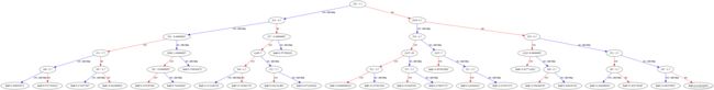
e)XGBOOST模型树

项目数据：
有人需要的话再发。。，会删除中文说明特殊处理